A Practical Guide to Transfer Learning using PyTorch
In this article, we’ll learn to adapt pre-trained models to custom classification tasks using a technique called transfer learning. We will demonstrate it for an image classification task using PyTorch, and compare transfer learning on 3 pre-trained models, Vgg16, ResNet50, and ResNet152.
Co-authored with Naresh and Gaurav.
This article will cover the what, why, and how of transfer learning.
- What is transfer learning
- Why should you use transfer learning
- How can you use transfer learning on a real classification task
Specifically, we’ll be covering the following aspects of transfer learning.
- The motivation behind the idea of transfer learning and its benefits.
- Develop an intuition for base model selection. (notebook)
- Discuss different choices and the trade-offs made along the way.
- Implementation of an image classification task with PyTorch. (notebook)
- Performance comparison of various base models.
- Resources to learn more about transfer learning and the current state of the art
Transfer learning is a large and growing field and this article covers just a few of its aspects. However, there are many deep learning online communities which discuss transfer learning. For example, here is a good article on how we can leverage transfer learning to reach higher benchmarks than training models from scratch.
Intended Audience and Prerequisites
- You’re familiar with basic machine learning (ML) concepts such as defining and training classification models
- You’re familiar with PyTorch and torchvision
In the next section, we'll formally introduce transfer learning and explain it with examples.
What is transfer learning?
From this page,
“Transfer learning is a machine learning method where a model developed for a task is reused as the starting point for a model on a second task.”
A deep learning model is a network of weights whose values are optimized using a loss function during the training progress. The weights of the network are typically initialized randomly before the start of the training process. In transfer learning, we use a pre-trained model that has been trained on a related task. This gives us a set of initial weights that are likely to perform better than the randomly initialized weights. We optimize the pre-trained weights further for our specific task.
Jeremy Howard (from fast.ai) says.
“Wherever possible, you should aim to start your neural network training with a pre-trained model and fine-tune it. You really don’t want to be starting with random weights, because that means that you’re starting with a model that doesn’t know how to do anything at all! With pretraining, you can use 1000x less data than starting from scratch.”
Below, we’ll see how one can think of the concept of transfer learning as it relates to humans.
Human Analogy for Transfer Learning
- Model training: After a child is born, it takes them a while to learn to stand, balance, and walk. During this time, they go through the phase of building physical muscles, and their brain learns to understand and internalize the skills to stand, balance and walk. They go through several attempts, some successful and some failures, to reach a stage where they can stand, balance and walk with some consistency. This is similar to training a deep learning model which takes a lot of time (training epochs) to learn a generic task (such as classifying an image as belonging to one of the 1000 ImageNet classes) when it is trained on that task.
- Transfer learning: A child who has learned to walk finds it far easier to learn related advanced skills such as jumping and running. Transfer Learning is comparable to this aspect of human learning where a pre-trained model that has already learned generic skills is leveraged to efficiently train for other related tasks.
Now that we have built an intuitive understanding of transfer learning and an analogy with human learning, let’s take a look at why one would use transfer learning for ML models.
Why should I use transfer learning?
Many vision AI tasks such as image classification, image segmentation, object localization, or detection differ only in the specific objects they are classifying, segmenting, or detecting. The models trained on these tasks have learned the features of the objects in their training dataset. Hence, they can be easily adapted to related tasks. For example, a model trained to identify the presence of a car in an image could be fine-tuned for identifying a cat or a dog.
The main advantage of transfer learning is the ability to empower you to achieve better accuracy on your tasks. We can break down its advantages as follows:
- Training efficiency: When you start with a pre-trained model that has already learned the general features of the data, you then only need to fine-tune the model to your specific task, which can be done much more quickly (i.e. using fewer training epochs).
- Model accuracy: Using transfer learning can give you a significant performance boost compared to training a model from scratch using the same amount of resources. Choosing the right pre-trained model for transfer-learning for your specific task is important though.
- Training data size: Since a pre-trained model would have already learned to identify many of the features that overlap with your task-specific features, you can train the pre-trained model with less domain-specific data. This is useful if you don’t have as much labeled data for your specific task.
So, how do we go about doing transfer learning in practice? The next section implements transfer learning in PyTorch for a flower classification task.
Transfer Learning with PyTorch
To perform transfer learning with PyTorch, we first need to select a dataset and a pre-trained vision model for image classification. This article focuses on using torch-vision (a domain library used with PyTorch). Let’s understand where to find such pre-trained models and datasets.
Where to find pre-trained vision models for image classification?
There are lots of websites providing high-quality pre-trained image classification models. For example:
For the purposes of this article, we will use pre-trained models from torchvision. It's worth learning a bit about how these models were trained. Let's explore that question next!
Which datasets are torchvision models pre-trained on?
For vision-related tasks involving images, torchvision models are usually pre-trained on the ImageNet dataset. The most popular ImageNet subset used by researchers and for model pre-training vision models contains about 1.2M images across 1000 classes. ImageNet classification is used as a pre-training task due to:
- Its ready availability to the research community
- The breadth and variety of images it contains
- Its use by various researchers - making it attractive to compare results using a common denominator of Imagenet 1k classification
You can read more about the history of the ImageNet challenge, historical background, and information about the complete dataset on this wikipedia page.
Legality considerations when using pre-trained models
ImageNet is released for non-commercial research purposes only (https://image-net.org/download). Hence, it’s not clear if one can legally use the weights from a model that was pre-trained on ImageNet for commercial purposes. If you plan to do so, please seek legal advice.
Now that we know where we can find the pre-trained models we’ll be using for transfer learning, let’s take a look at where we can procure the dataset we wish to use for our custom classification task.
Dataset: Oxford Flowers 102
We will be using the Flowers 102 dataset to illustrate transfer learning using PyTorch. We will train a model to classify images in the Flowers 102 dataset into one of the 102 categories. This is a multi-class (single-label) categorization problem in which predicted classes are mutually exclusive. We’ll be leveraging Torchvision for this task since it already provides this dataset for us to use.
The Flowers 102 dataset was obtained from the Visual Geometry Group at Oxford. Please see the page for licensing terms for the use of the dataset.
Next, let’s take a look at the high-level steps involved in this process.
How does transfer learning work?
Transfer learning for image classification tasks can be viewed as a sequence of three steps as shown in Figure 1. These steps are as follows:
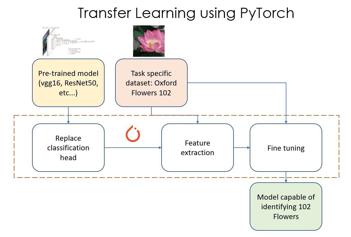
Figure 1: Transfer Learning using PyTorch. Source: Author(s)
- Replace classifier layer: In this phase, we identify and replace the last “classification head” of our pre-trained model with our own “classification head” that has the right number of output features (102 in this example).
- Feature extraction: In this phase, we freeze (make those layers non-trainable) all the layers of the model except the newly added classification layer, and train just this newly added layer.
- Fine tuning: In this phase, we unfreeze some subset of the layers in the model (unfreezing a layer means making it trainable). In this article, we will unfreeze all the layers of the model and train them as we would train any Machine Learning (ML) PyTorch model.
Each of these phases has a lot of additional detail and nuance that we need to know and worry about. We’ll get into those details soon. For now, let’s deep dive into 2 of the key phases, namely feature extraction, and fine-tuning below.
Feature extraction and fine-tuning
You can find more information about feature extraction and fine-tuning here.
- What is the difference between feature extraction and fine-tuning in transfer learning?
- Learning without forgetting
The diagrams below illustrate feature extraction and fine tuning visually.
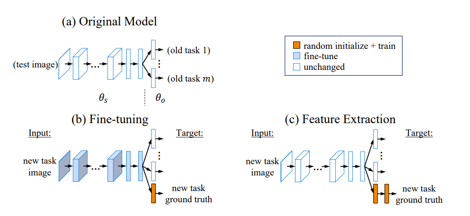
Figure 2: Visual explanation of fine tuning (b) and feature extraction (c). Source: Learning without forgetting
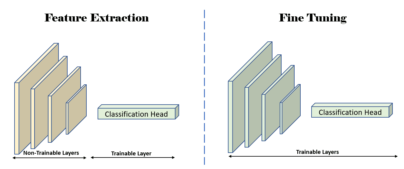
Figure 3: Illustration showing which layers are trainable (unfrozen) during the feature-extraction, and fine-tuning stages. Source: Author(s)
Now that we’ve developed a good understanding of the custom classification task, the pre-trained model we’ll be using for this task, and how transfer learning works, let’s look at some concrete code that performs transfer learning.
Show me the Code
In this section you will learn concepts like exploratory model analysis, initial model selection, how to define a model, implement transfer learning steps (discussed above), and how to prevent overfitting. We’ll discuss the train/val/test split for this dataset and interpret the results.
The complete code for this experiment can be found here (Flowers102 classification using pre-trained models). The section on exploratory model analysis is in a separate notebook.
Exploratory model analysis
Similar to exploratory data analysis in data science, the first step in transfer-learning is exploratory model analysis. In this step, we explore all the pre-trained models available for image classification tasks, and determine how each one is structured.
In general, it’s hard to know which model will perform best for our task, so it’s not uncommon to try out a few models that seem promising or applicable for our situation. In this hypothetical scenario, let’s assume that model size isn’t important (we don’t want to deploy these models on mobile devices or such edge devices). We’ll first look at the list of available pre-trained classification models in torchvision.
classification_models = torchvision.models.list_models(module=torchvision.models)

print(len(classification_models), "classification models:", classification_models)
Will print
80 classification models: ['alexnet', 'convnext_base', 'convnext_large', 'convnext_small', 'convnext_tiny', 'densenet121', 'densenet161', 'densenet169', 'densenet201', 'efficientnet_b0', 'efficientnet_b1', 'efficientnet_b2', 'efficientnet_b3', 'efficientnet_b4', 'efficientnet_b5', 'efficientnet_b6', 'efficientnet_b7', 'efficientnet_v2_l', 'efficientnet_v2_m', 'efficientnet_v2_s', 'googlenet', 'inception_v3', 'maxvit_t', 'mnasnet0_5', 'mnasnet0_75', 'mnasnet1_0', 'mnasnet1_3', 'mobilenet_v2', 'mobilenet_v3_large', 'mobilenet_v3_small', 'regnet_x_16gf', 'regnet_x_1_6gf', 'regnet_x_32gf', 'regnet_x_3_2gf', 'regnet_x_400mf', 'regnet_x_800mf', 'regnet_x_8gf', 'regnet_y_128gf', 'regnet_y_16gf', 'regnet_y_1_6gf', 'regnet_y_32gf', 'regnet_y_3_2gf', 'regnet_y_400mf', 'regnet_y_800mf', 'regnet_y_8gf', 'resnet101', 'resnet152', 'resnet18', 'resnet34', 'resnet50', 'resnext101_32x8d', 'resnext101_64x4d', 'resnext50_32x4d', 'shufflenet_v2_x0_5', 'shufflenet_v2_x1_0', 'shufflenet_v2_x1_5', 'shufflenet_v2_x2_0', 'squeezenet1_0', 'squeezenet1_1', 'swin_b', 'swin_s', 'swin_t', 'swin_v2_b', 'swin_v2_s', 'swin_v2_t', 'vgg11', 'vgg11_bn', 'vgg13', 'vgg13_bn', 'vgg16', 'vgg16_bn', 'vgg19', 'vgg19_bn', 'vit_b_16', 'vit_b_32', 'vit_h_14', 'vit_l_16', 'vit_l_32', 'wide_resnet101_2', 'wide_resnet50_2']
Wow! That’s a pretty large list of models to choose from! If you’re feeling confused, don’t worry - in the next section, we’ll look at the factors to consider when choosing the initial set of models for performing transfer learning.
Initial model selection
Now that we have a list of 80 candidate models to choose from, we need to narrow it down to a handful of models that we can run experiments on. The choice of the pre-trained model backbone is a hyper-parameter, and we can (and should) explore multiple options by running experiments to see which one works best. Running experiments is costly and time consuming, and it’s unlikely that we’ll be able to try all the models, which is why we try to narrow down the list to 3-4 models to begin with.
We decided to go with the following pre-trained model backbones to begin with.
- Vgg16: 135M parameters
- ResNet50: 23M parameters
- ResNet152: 58M parameters
Here’s how/why we chose these 3 to begin with.
- We’re not constrained by model size or inference latency, so we don’t need to find the models that are super efficient. If you want a comparative study of various vision models for mobile devices, please read the paper titled “Comparison and Benchmarking of AI Models and Frameworks on Mobile Devices”.
- The models we choose are fairly popular in the vision ML community and tend to be good go-to choices for classification tasks. You could use the citation count for papers on these models as decent proxies for how effective these models could be. However, please be aware of a potential bias where papers on models such as AlexNet that have been around long will have more citations even though one would not use them for any serious classification task as a default choice.
- Even within model architectures, there tend to be many flavours or sizes of models. For example, EfficientNet comes in trims named B0 through B7. Please refer to the papers on the specific models for details on what these trims mean.
Citation counts of various papers on pre-trained classification models available in torchvision.
- Resnet: 165k
- AlexNet: 132k
- Vgg16: 102k
- MobileNet: 19k
- Vision Transformers: 16k
- EfficientNet: 12k
- ShuffleNet: 6k
If you’d like to read more on factors that may affect your choice of pre-trained model, please read the following articles:
- 4 Pre-Trained CNN Models to Use for Computer Vision with Transfer Learning
- How to choose the best pre-trained model for your Convolutional Neural Network?
- Benchmark Analysis of Representative Deep Neural Network Architectures
Let’s check out the classification heads for these models.
vgg16 = torchvision.models.vgg16_bn(weights=None)
resnet50 = torchvision.models.resnet50(weights=None)
resnet152 = torchvision.models.resnet152(weights=None)

print("vgg16\n", vgg16.classifier)
print("resnet50\n", resnet50.fc)
print("resnet152\n", resnet152.fc)
vgg16
 Sequential(
  (0): Linear(in_features=25088, out_features=4096, bias=True)
  (1): ReLU(inplace=True)
  (2): Dropout(p=0.5, inplace=False)
  (3): Linear(in_features=4096, out_features=4096, bias=True)
  (4): ReLU(inplace=True)
  (5): Dropout(p=0.5, inplace=False)
  (6): Linear(in_features=4096, out_features=1000, bias=True)
)
resnet50
 Linear(in_features=2048, out_features=1000, bias=True)
resnet152
 Linear(in_features=2048, out_features=1000, bias=True)
You can find the complete notebook for exploratory model analysis here.
Since we’re going to be running experiments on 3 pre-trained models and performing transfer learning on each one of them separately, let’s define some abstractions and classes that will help us run and track these experiments.
Defining a PyTorch model to wrap pre-trained models
To allow easy exploration, we will define a PyTorch model named Flowers102Classifier, and use that throughout this exercise. We will progressively add functionality to this class till we achieve our final goal. The complete notebook for transfer learning for Flowers 102 classification can be found here.
The sections below will dive deeper into each of the mechanical steps needed to perform transfer learning.
Replacing the old classification head with a new one
The existing classification head for each of these models that is pre-trained on the ImageNet classification task has 1000 output features. Our custom task for flower classification has 102 output features. Hence, we need to replace the final classification head (layer) with a new one that has 102 output features.
The constructor for our class will include code that loads the pre-trained model of interest from torchvision using pre-trained weights, and will replace the classification head with a custom classification head for 102 classes.
def __init__(self, backbone, load_pretrained):
    super().__init__()
    assert backbone in backbones
    self.backbone = backbone
    self.pretrained_model = None
    self.classifier_layers = []
    self.new_layers = []

    if backbone == "resnet50":
        if load_pretrained:
            self.pretrained_model = torchvision.models.resnet50(
                weights=torchvision.models.ResNet50_Weights.IMAGENET1K_V2
            )
        else:
            self.pretrained_model = torchvision.models.resnet50(weights=None)
        # end if

        self.classifier_layers = [self.pretrained_model.fc]
        # Replace the final layer with a classifier for 102 classes for the Flowers 102 dataset.
        self.pretrained_model.fc = nn.Linear(
            in_features=2048, out_features=102, bias=True
        )
        self.new_layers = [self.pretrained_model.fc]
    elif backbone == "resnet152":
        if load_pretrained:
            self.pretrained_model = torchvision.models.resnet152(
                weights=torchvision.models.ResNet152_Weights.IMAGENET1K_V2
            )
        else:
            self.pretrained_model = torchvision.models.resnet152(weights=None)
        # end if

        self.classifier_layers = [self.pretrained_model.fc]
        # Replace the final layer with a classifier for 102 classes for the Flowers 102 dataset.
        self.pretrained_model.fc = nn.Linear(
            in_features=2048, out_features=102, bias=True
        )
        self.new_layers = [self.pretrained_model.fc]
    elif backbone == "vgg16":
        if load_pretrained:
            self.pretrained_model = torchvision.models.vgg16_bn(
                weights=torchvision.models.VGG16_BN_Weights.IMAGENET1K_V1
            )
        else:
            self.pretrained_model = torchvision.models.vgg16_bn(weights=None)
        # end if

        self.classifier_layers = [self.pretrained_model.classifier]
        # Replace the final layer with a classifier for 102 classes for the Flowers 102 dataset.
        self.pretrained_model.classifier[6] = nn.Linear(
            in_features=4096, out_features=102, bias=True
        )
        self.new_layers = [self.pretrained_model.classifier[6]]
Since we’ll be performing feature-extraction followed by fine-tuning, we’ll save the newly added layers into the self.new_layers list. This will help us set the weights of those layers as trainable or non-tainable depending on what we’re doing.
Now that we have replaced the older classification head with a new classification head that has randomly initialized weights, we will need to train those weights so that the model can perform accurate predictions. This includes feature extraction and fine tuning and we’ll take a look at that next.
Transfer Learning (trainable parameters and learning rates)
Transfer learning involves running feature extraction and fine tuning in that specific order. Let’s take a closer look at why they need to be run in that order and how we can handle trainable parameters for the various transfer learning phases.
Feature Extraction: We set requires_grad to False for weights in all the layers in the model, and set requires_grad to True for only the newly added layers.
We train the new layer(s) for 16 epochs with a learning rate of 1e-3. This ensures that the new layer(s) are able to adjust and adapt their weights to the weights in the feature extractor part of the network. It’s important to freeze the rest of the layers in the network and train only the new layer(s) so that we don’t shock the network into forgetting what it has already learned. If we don’t freeze the earlier layers, they will end up getting re-trained on junk weights that were randomly initialized when we added the new classification head.
Fine Tuning: We set requires_grad to True for weights in all the layers of the model. We train the entire network for 8 epochs. However, we adopt a differential learning rate strategy in this case. We decay the learning rate (LR) so that the LR decreases as we move toward the input layers (away from the output classification head). We decay the learning rate as we move up the model towards the initial layers of the model because those initial layers have learned basic features about the image, which would be common for most vision AI tasks. Hence, the initial layers are trained with a very low LR to avoid disturbing what they have learned. As we move down the model towards the classification head, the model is learning something task specific, so it makes sense to train those later layers with a higher LR. One can adopt different strategies here, and in our case, we use 2 different strategies to illustrate the effectiveness of both of them.
- VGG16: For the vgg16 network, we decay the LR linearly from LR=1e-4 to LR=1e-7 (1000x lower than the LR of the classification layer). Since there are 44 layers in the feature extraction phase, each layer is assigned a LR that is (1e-7 - 1e-4)/44 = 2.3e-6 lower than the previous layer.
- ResNet: For the ResNet (50/152) network, we decay the LR exponentially starting from LR=1e-4. We reduce the LR by 3x for every layer we move up.
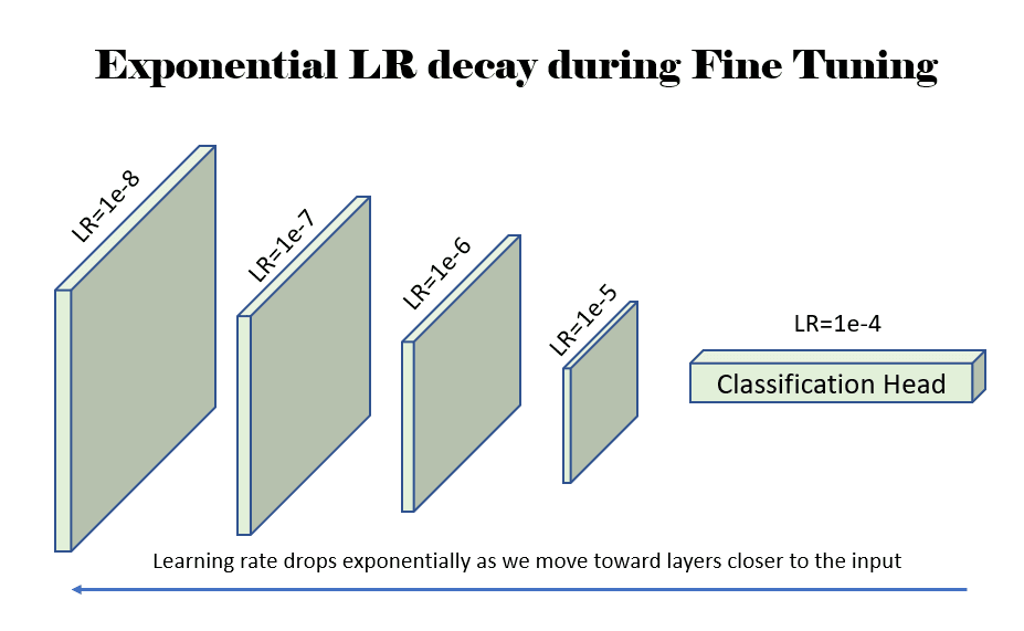
Figure 4: An example showing the learning rate (LR) decaying exponentially by a factor of 10 as we move up toward the layers closer to the input to the network. Source: Author(s).
The code for freezing layers for both feature extraction as well as fine tuning is shown in the function named fine_tune() below.
def fine_tune(self, what: FineTuneType):
    # The requires_grad parameter controls whether this parameter is
    # trainable during model training.
    m = self.pretrained_model
    for p in m.parameters():
        p.requires_grad = False
    if what is FineTuneType.NEW_LAYERS:
        for l in self.new_layers:
            for p in l.parameters():
                p.requires_grad = True
    elif what is FineTuneType.CLASSIFIER:
        for l in self.classifier_layers:
            for p in l.parameters():
                p.requires_grad = True
    else:
        for p in m.parameters():
            p.requires_grad = True
In PyTorch, the way to set differential LRs for each layer is to specify the weights that need that LR to the optimizer that will be used during transfer learning. In our notebook, we use the Adam optimizer. The get_optimizer_params() method below gets the optimizer parameters to pass into the Adam (or other) optimizer we will be using.
def get_optimizer_params(self):
    """This method is used only during model fine-tuning when we need to
    set a linearly or exponentially decaying learning rate (LR) for the
    layers in the model. We exponentially decay the learning rate as we
    move away from the last output layer.
    """
    options = []
    if self.backbone == "vgg16":
        # For vgg16, we start with a learning rate of 1e-3 for the last layer, and
        # decay it to 1e-7 at the first conv layer. The intermediate rates are
        # decayed linearly.
        lr = 0.0001
        options.append(
            {
                "params": self.pretrained_model.classifier.parameters(),
                "lr": lr,
            }
        )
        final_lr = lr / 1000.0
        diff_lr = final_lr - lr
        lr_step = diff_lr / 44.0
        for i in range(43, -1, -1):
            options.append(
                {
                    "params": self.pretrained_model.features[i].parameters(),
                    "lr": lr + lr_step * (44 - i),
                }
            )
        # end for
    elif self.backbone in ["resnet50", "resnet152"]:
        # For the resnet class of models, we decay the LR exponentially and reduce
        # it to a third of the previous value at each step.
        layers = ["conv1", "bn1", "layer1", "layer2", "layer3", "layer4", "fc"]
        lr = 0.0001
        for layer_name in reversed(layers):
            options.append(
                {
                    "params": getattr(self.pretrained_model, layer_name).parameters(),
                    "lr": lr,
                }
            )
            lr = lr / 3.0
        # end for
    # end if
    return options


# end def
Once we have the model parameters with their own LRs, we can pass them into the optimizer with a single line of code. A default LR of 1e-8 is used for parameters whose weights are not specified in the dictionary returned by get_optimizer_params().
optimizer = torch.optim.Adam(fc.get_optimizer_params(), lr=1e-8)Now that we know how to perform transfer learning, let’s take a look at what other considerations we need to keep in mind before we fine tune our model. This includes steps that we need to take to prevent overfitting, and choosing the right train/val/test split.
Preventing overfitting
In our notebook, we use the following data augmentation techniques on the training data to prevent overfitting and allow the model to learn the features so that it can perform predictions on unseen data.
- Color Jitter
- Horizontal Flip
- Rotation
- Shear
There is no data augmentation applied to the validation split.
One should also explore weight decaying, which is a regularization technique to prevent overfitting by reducing the complexity of the model.
Train/Val/Test split
The authors of the Flowers 102 dataset recommend a train/val/test split that’s of size 1020/ 1020/6149. Many authors do things differently. For example,
- In the ResNet strikes back paper, the authors use the train+val (2040 images) split as the train set, and the test set as the test set. It isn’t clear if there’s a validation split.
- In this article on classification on Flowers 102, the authors use the test split of size 6149 as the train split.
- In this notebook, the author uses a train/val/test split of size 6552, 818, and 819 respectively.
The only way to know which author is doing what is to read the papers or the code.
In our notebook (in this article), we use the split of size 6149 as the train split and the split of size 2040 as the validation split. We don’t use a test split, since we aren’t really trying to compete here.
At this point in time, you should feel empowered to visit this notebook that performs all of the steps above and has their results presented for you to view. Please feel free to clone the notebook on Kaggle or Google Colab and run it yourself on a GPU. If you’re using Google Colab, you’ll need to fix up some of the paths where the datasets and pre-trained models are downloaded and where the best weights for the fine-tuned models are stored.
Below, we will look at the results of our transfer learning experiments!
Results
The results have some common themes that we’ll explore below.
- After the feature extraction step alone, almost all the networks have an accuracy between 91% and 94%
- Almost all networks do really well, achieving an accuracy of 96+% after the fine-tuning step. This shows that the fine tuning step really helps during transfer learning.
There’s a significant difference in the number of parameters in our network, with vgg16 at 135M parameters, ResNet50 at 23M parameters, and ResNet152 at 58M parameters. This suggests that we can probably find a smaller network with comparable accuracy and performance.
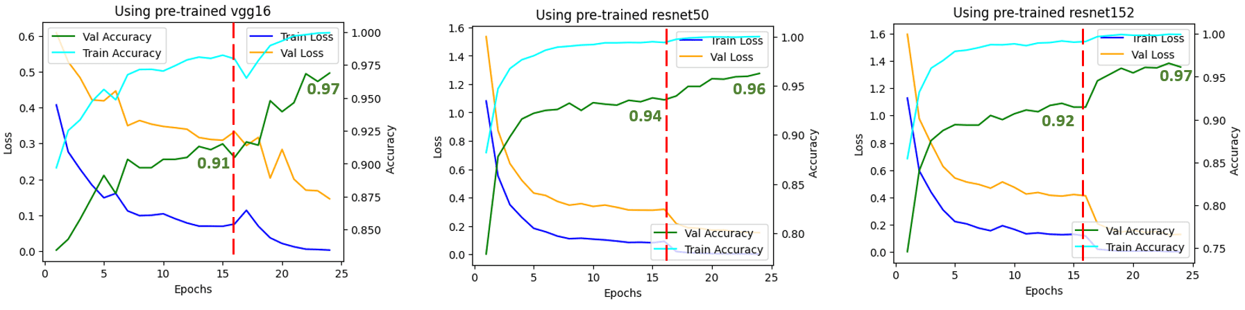
Figure 5: Train/Val Loss and Accuracy over the transfer learning process. Source: Author(s).
The vertical red line indicates the epoch when we switched from feature extraction (16 epochs) to fine-tuning (8 epochs). You can see that when we switched to fine-tuning, all the networks showed an increase in accuracy. This shows that fine-tuning after feature extraction is very effective.
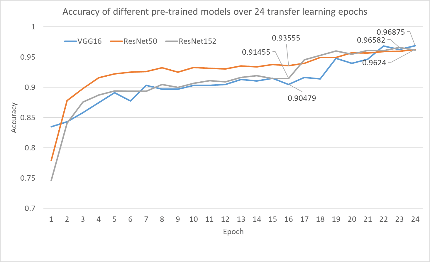
Figure 6: Validation accuracy of all the 3 pre-trained models after transfer learning on the flowers classification task. The validation accuracy after feature extraction at epoch 16 is shown along with the best validation accuracy for each model during the fine tuning phase. Source: author(s).
Article Recap
- Transfer learning is a thrifty and effective way to train your network by starting from a pre-trained network on a similar but unrelated task
- Torchvision provides many models pre-trained on ImageNet for researchers to use during transfer learning
- Be careful when using pre-trained models in production to ensure that you don’t violate any licenses or terms of use for datasets on which models were pre-trained
- Transfer learning includes feature extraction and fine-tune, which must be performed in that specific order
Want to learn more?
Now that we know how to perform transfer learning for a custom task starting from a model that is pre-trained on a different dataset, wouldn’t it be great if we could avoid using a separate dataset for the pre-training (pretext task) and use our own dataset for this purpose? Turns out, this is becoming feasible!
Recently, researchers and practitioners have been using self-supervised learning as a way to perform model pre-training (learning the pretext task) which has a benefit of training the model on a dataset with the same distribution as the target dataset that the model is supposed to be consuming in production. If you are interested in learning more about self-supervised pre-training and hierarchical pretraining, please see this paper from 2021 titled self-supervised pretraining improves self-supervised pretraining.
If you own the data for your specific task, you can use self-supervised learning for pre-training your model and not worry about using the ImageNet dataset for the pre-training step, thus staying in the clear as far as use of the ImageNet dataset is concerned.
Glossary of Terms used
- Classification head: In PyTorch, this is an nn.Linear layer that maps numerous input features to a set of output features
- Freeze weights: Make the weights non-trainable. In PyTorch, this is done by setting requires_grad=False
- Unfreeze (or thaw) weights: Make the weights trainable. In PyTorch, this is done by setting requires_grad=True
- Self-supervised learning: A way to train an ML model so that it can be trained on data without any human generated labels. The labels could be automatically or machine generated though
References and Further Reading
- Ideas on how to fine-tune a pre-trained model in PyTorch
- Dive into deep learning: Fine tuning
- Self-supervised learning and computer vision
- A Gentle Introduction to Transfer Learning for Deep Learning
- Notebook: Exploratory model analysis
- Notebook: Flowers 102 classification using transfer learning
Dhruv Matani is a Machine Learning enthusiast focusing on PyTorch, CNNs, Vision, Speech, and Text AI. He is an expert on on-device AI, model optimization and quantization, ML and Data Infrastructure. Authoring a chapter on Efficient PyTorch in the Efficient Deep Learning Book at https://efficientdlbook.com/. His views are his own, not those of any of his employer(s); past, present, or future.
Naresh is deeply interested in the "learning" aspect of the Neural Network. His work is focussed on neural network architectures and how simple topological changes enhance their learning capabilities. He has held engineering roles at Microsoft, Amazon, and Citrix in his decade-long professional career. He has been involved in the deep learning field for the last 6-7 years. You can find him on medium at https://medium.com/u/1e659a80cffd.
Gaurav is a Staff Software Engineer at Google Research where he leads research projects geared towards optimizing large machine learning models for efficient training and inference on devices ranging from tiny microcontrollers to Tensor Processing Unit (TPU)-based servers. His work has positively impacted over 1 Billion of active users across YouTube, Cloud, Ads, Chrome, etc. He is also an author of an upcoming book with Manning Publication on Efficient Machine Learning. Before Google, Gaurav worked at Facebook for 4.5 years and has contributed significantly to Facebook’s Search system and large-scale distributed databases. He has an M.S. in Computer Science from Stony Brook University.