Using RAPIDS cuDF to Leverage GPU in Feature Engineering
Improving Performance by Replacing Pandas with cuDF in Creating Data Frames and Engineering Features and Integrating with Google Colab.
Editor's note: This was the runner-up in our recent NVIDIA + KDnuggets GPU-themed blog writing contest. Congratulations to Hasan on the accomplishment!
The fact that particular methods succeeded in solving a problem may not lead to the same outcome on a different scale. When distances change, shoes need to change too.
In machine learning, data, and data processing are crucial in ensuring the model’s success, and feature engineering is part of that process. When the data is small, the classical Pandas library can easily handle any processing task on the CPU. However, Pandas can be too slow in processing big data. One solution to improving speed and efficiency in data processing and feature engineering is RAPIDS.
“RAPIDS is a suite of open-source software libraries for executing end-to-end data science and analytics pipelines entirely on graphics processing units (GPUs). RAPIDS accelerates data science pipelines to create more productive workflows.[1]”

Image by brgfx on Freepik
One tool by RAPIDS to efficiently manipulate tabular data in feature engineering and data preprocessing is cuDF. RAPIDS cuDF enables the creation of GPU data frames and the performance of several Pandas operations such as indexing, groupby, merging, and string handling. As the RAPIDS website defines:
“cuDF is a Python GPU DataFrame library (built on the Apache Arrow columnar memory format) for loading, joining, aggregating, filtering, and otherwise manipulating tabular data using a DataFrame style API in the style of pandas.[2]”
This article tries to explain how to create and manipulate data frames and apply feature engineering with cuDF on GPU using a real dataset.
Our dataset belongs to Optiver Realized Volatility Prediction of Kaggle. It contains stock market data relevant to the practical execution of trades in the financial markets and includes order book snapshots and executed trades[3].
We’ll discover more about the data in the following section. Then, we will integrate Google Colab with Kaggle and RAPIDS. In the third section, we will see how to accomplish feature engineering on this dataset using Pandas and cuDF. That will provide us with a comparative performance review of both libraries. In the last section, we will plot and evaluate the results.
Data
The data we are going to use consists of two sets of files[3]:
- book_[train/test].parquet: A parquet file, which is partitioned by stock_id, provides order book data on the most competitive buy and sell orders entered into the market. This file contains passive buy/sell intention updates.
Feature columns in book_[train/test].parquet:
- stock_id - ID code for the stock. Parquet coerces this column to the categorical data type when loaded.
- time_id - ID code for the time bucket. Time IDs are not necessarily sequential but are consistent across all stocks.
- seconds_in_bucket - Number of seconds from the start of the bucket, always starting from 0.
- bid_price[1/2] - Normalized prices of the most/second most competitive buy level.
- ask_price[1/2] - Normalized prices of the most/second most competitive sell level.
- bid_size[1/2] - The number of shares on the most/second most competitive buy level.
- ask_size[1/2] - The number of shares on the most/second most competitive sell level.
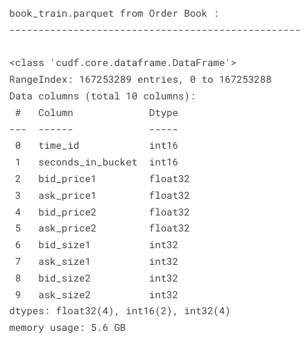
Exhibit-1: Description of book_[train/test].parquet (Image by Author)
This file is 5.6 GB and contains more than 167 million entries. There are 112 stocks and 3830 10-minute time windows (time_id). Each time window (bucket) has a maximum of 600 seconds. As one transaction intention can occur per second in each time window for each stock, the multiplication of the mentioned numbers can explain why we have millions of entries. A caveat is that not every second a transaction intention occurs, meaning that some seconds in a particular time window are missing.
- trade_[train/test].parquet: A parquet file, which is partitioned by stock_id, contains data on trades that are actually executed.
Feature columns in trade_[train/test].parquet:
- stock_id - Same as above.
- time_id - Same as above.
- seconds_in_bucket - Same as above. Note that since trade and book data are taken from the same time window and trade data is more sparse in general, this field is not necessarily starting from 0.
- price - The average price of executed transactions happening in one second. Prices have been normalized and the average has been weighted by the number of shares traded in each transaction.
- size - The total number of shares traded.
- order_count - The number of unique trade orders taking place.
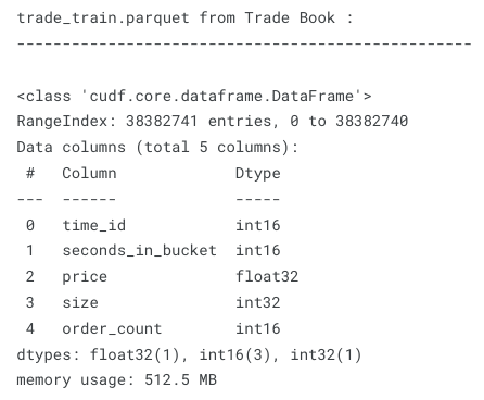
Exhibit-2: Description of trade_[train/test].parquet (Image by Author)
The trade_[train/test].parquet file is much less than book_[train/test].parquet. The former is 512.5 MB and has more than 38 million entries. Since actual transactions don’t have to match intentions, trade data is more sparse and hence fewer entries.
The goal is to predict the realized stock price volatility computed over the next 10-minute window from the feature data under the same stock_id/time_id. This project involves a great deal of feature engineering that should be performed on a large dataset. Developing new features will also increase the size of the data and the computational complexity. One remedy is to use cuDF instead of the Pandas library.
In this blog, we will see a few feature engineering tasks and data frame manipulations trying both Pandas and cuDF to compare their performances. However, we won’t use all the data but only a single stock’s records to see an exemplary implementation. One may check out the notebook to see all feature engineering work done on the entire data.
Since we execute the code on Google Colab, we should first configure our notebook to integrate Kaggle and RAPIDS.
Configuration of Google Colab Notebook
There are a few steps to configure the Colab notebook:
- Create an API token on the Kaggle account to authenticate the notebook with Kaggle services.
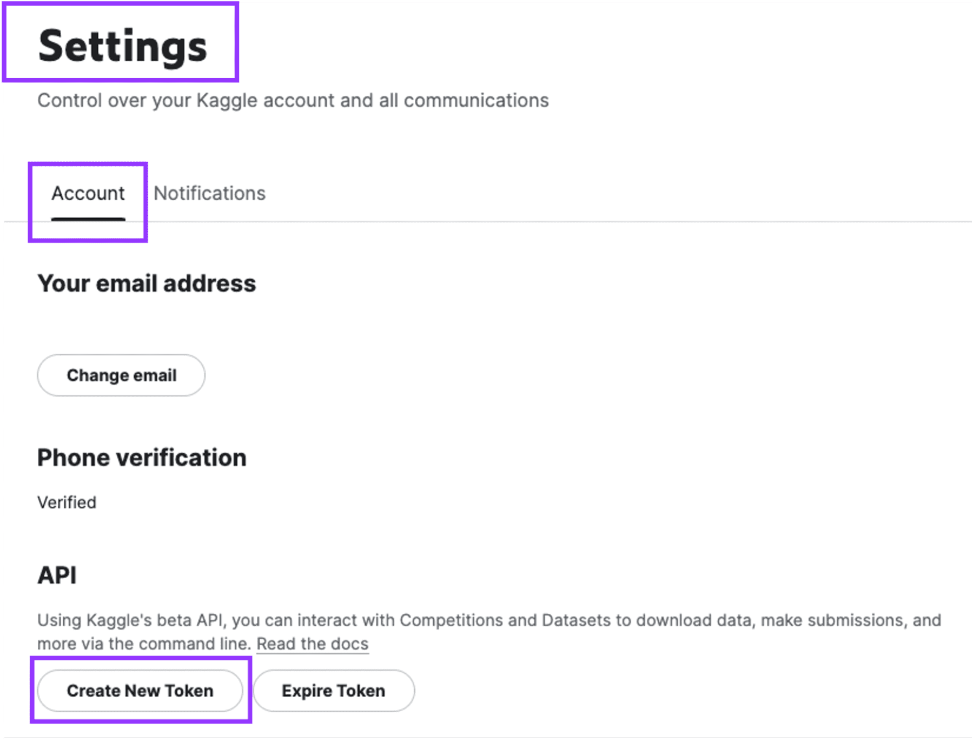
Exhibit-3: Creating An API Token On The Kaggle Account (Image by Author)
Go to Settings and click on “Create New Token.” A file named “kaggle.json” will be downloaded which contains the username and the API key.
- Start a new notebook on Google Colab and upload the kaggle.json file.
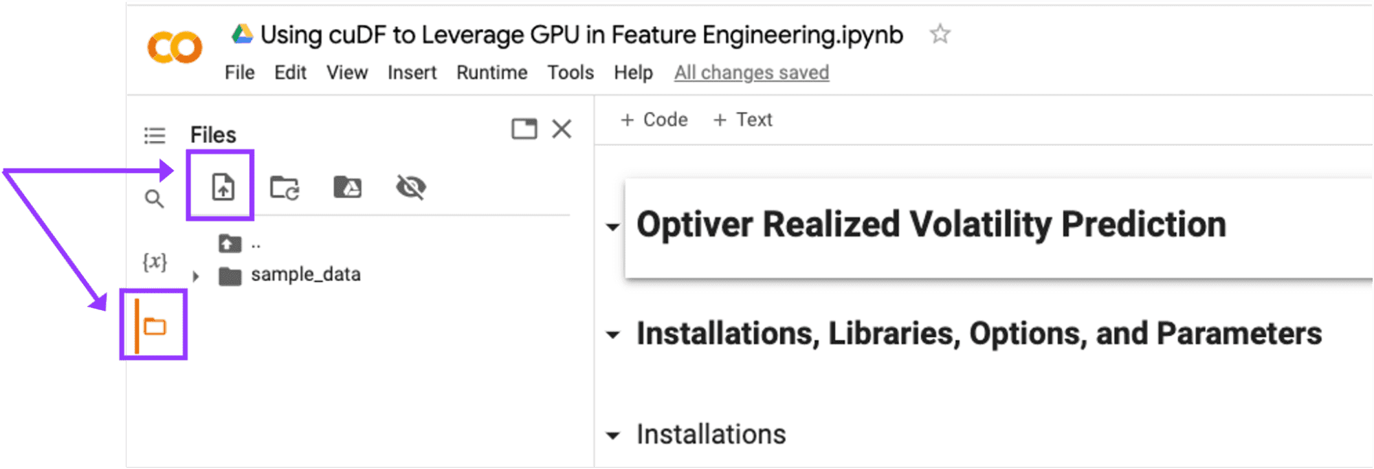
Exhibit-4: Uploading The kaggle.json File In Google Colab (Image by Author)
Upload the kaggle.json file in Google Colab by clicking on the “Upload to session storage” icon.
- Click the “Runtime” dropdown at the top of the page, then “Change Runtime Type” and confirm the instance type is GPU.
- Execute the below command and check the output to ensure you have been allocated a Tesla T4, P4, or P100.
!nvidia-smi
- Get RAPIDS-Colab install-files and check your GPU:
!git clone https://github.com/rapidsai/rapidsai-csp-utils.git
!python rapidsai-csp-utils/colab/pip-install.py
Ensure that your Colab Instance is RAPIDS compatible in the output of this cell.
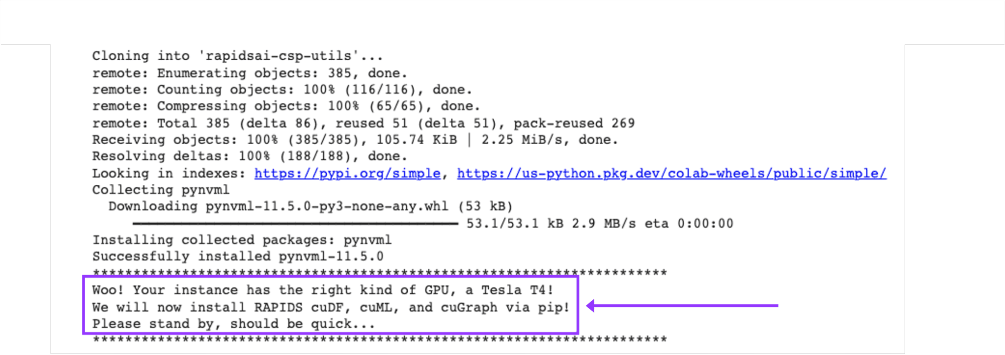
Exhibit-5: Checking If The Colab Instance Is RAPIDS Compatible (Image by Author)
- Check if RAPIDS libraries are installed correctly:
import cudf, cuml
cudf.__version__
We are all set with the Google Colab configuration if the setup renders no error. Now, we can upload the Kaggle dataset.
Importing and Uploading the Kaggle Dataset
We need to make a few arrangements in our Colab instance to import the dataset from Kaggle.
- Install the Kaggle library:
!pip install -q kaggle
- Make a directory named “.kaggle”:
!mkdir ~/.kaggle
- Copy the “kaggle.json” into this new directory:
!cp kaggle.json ~/.kaggle/
- Allocate the required permission for this file:
!chmod 600 ~/.kaggle/kaggle.json
- Download the dataset from Kaggle:
!kaggle competitions download optiver-realized-volatility-prediction
- Create a directory for unzipped data:
!mkdir train
- Unzip data in the new directory:
!unzip optiver-realized-volatility-prediction.zip -d train
- Import all other libraries we need:
import glob
import numpy as np
import pandas as pd
from cudf import DataFrame
import matplotlib.pyplot as plt
from matplotlib import style
from collections import defaultdict
from IPython.display import display
import gc
import time
import warnings
%matplotlib inline
- Set Pandas options:
pd.set_option("display.max_colwidth", None)
pd.set_option("display.max_columns", None)
warnings.filterwarnings("ignore")

print("Threshold:", gc.get_threshold())
print("Count:", gc.get_count())
- Define parameters:
# Data directory that contains files
DIR = "/content/train/"

# Number of execution cycles
ROUNDS = 30
- Get files:
# Get order and trade books
order_files = glob.glob(DIR + "book_train.parquet" + "/*")
trade_files = glob.glob(DIR + "trade_train.parquet" + "/*")
print(order_files[:5])
print("\n")
print(trade_files[:5])
print("\n")

# Get stock_ids as a list
stock_ids = sorted([int(file.split('=')[1]) for file in order_files])
print(f"{len(stock_ids)} stocks: \n {stock_ids} \n")
Now, our notebook is ready to run all data frame tasks and perform feature engineering.
Feature Engineering
This section will discuss 13 typical engineering operations on Pandas data frame and cuDF. We will see how long these operations take and how much memory they use. Let us start by loading the data first.
1. Loading data
def load_dataframe(files, dframe=0):

   print("LOADING DATA FRAMES", "\n")

   # Load the pandas dataframe
   if dframe == 0:
     print("Loading pandas dataframe..", "\n")
     start = time.time()
     df_pandas = pd.read_parquet(files[0])
     end = time.time()
     elapsed_time = round(end-start, 3)
     print(f"For pandas dataframe: \n start time: {start} \n end time: {end} \n elapsed time: {elapsed_time} \n")
     return df_pandas, elapsed_time

   # Load the cuDF dataframe
   else:
     print("Loading cuDF dataframe..", "\n")
     start = time.time()
     df_cudf = cudf.read_parquet(files[0])
     end = time.time()
     elapsed_time = round(end-start, 3)
     print(f"For cuDF dataframe: \n start time: {start} \n end time: {end} \n elapsed time: {elapsed_time} \n ")

     return df_cudf, elapsed_time
When dframe=0, data will be loaded as a Pandas data frame, otherwise cuDF. For example,
Pandas:
# Load pandas order dataframe and calculate time
df_pd_order, _ = load_dataframe(order_files, dframe=0)
display(df_pd_order.head())
This will return the first five records of the Order Book (book_[train/test].parquet):
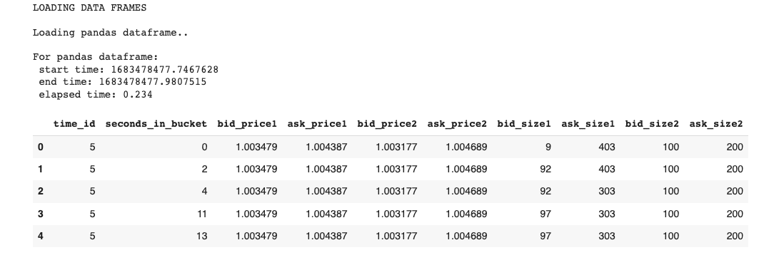
Exhibit-6: Loading The Data As Pandas Dataframe (Image by Author)
cuDF:
# Load cuDF book dataframe and calculate time
df_cudf_order, _ = load_dataframe(order_files, dframe=1)
display(df_cudf_order.head())
Output:
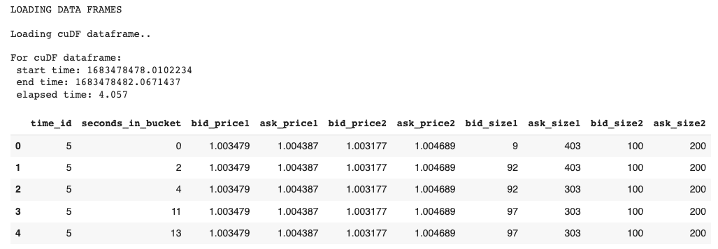
Exhibit-7: Loading The Data As cuDF (Image by Author)
Let us get information about the Order Book data from the Pandas version:
# Order dataframe info
display(df_pd_order.info())
Output:
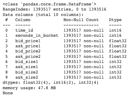
Exhibit-8: Information About The First Stock’s Order Book Data (Image by Author)
The above image tells us that the first stock has around 1.4 million entries and holds 47.8 MB of memory space. To reduce the space and increase the speed, we should convert data types to lesser formats, which we’ll do later.
In a similar fashion, we load the Trade Book (trade_[train/test].parquet) data in both data frame libraries as we did for the Order Book data. The data and its information will look like this:
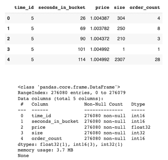
Exhibit-9: The First Stock’s Trade Book Data And Data Info (Image by Author)
The trading data for the first stock is 3.7 MB and has over 276 thousand records.
In both files (Order Book and Trade Book), not every time window has 600 points of seconds. In other words, a particular time bucket may have transactions or bids only on some seconds in the 10-minute interval. That makes us face sparse data in both files where some seconds are missing. We should fix it by forward-filling all columns for the missing seconds. While Pandas allows us to forward fill, cuDF doesn’t have that feature. Thus, we will do forward-filling in Pandas and re-create the cuDF from the forward-filled Pandas data frame. We feel remorse about this as the central goal of this blog is to show how cuDF outperforms Pandas. I checked into the matter multiple times in the past, but to the best knowledge, I couldn’t come across the method in cuDF as implemented in Pandas. Thus, we can do forward-filling as follows[4]:
# Forward fill data
def ffill(df, df_name="order"):

   # Forward fill
   df_pandas = df.set_index(['time_id', 'seconds_in_bucket'])

   if df_name == "order":
     df_pandas = df_pandas.reindex(pd.MultiIndex.from_product([df_pandas.index.levels[0], np.arange(0,600)], names = ['time_id', 'seconds_in_bucket']), method='ffill')
     df_pandas = df_pandas.reset_index()

   else:
     df_pandas = df_pandas.reindex(pd.MultiIndex.from_product([df_pandas.index.levels[0], np.arange(0,600)], names = ['time_id', 'seconds_in_bucket']))
     # Fill nan values with 0
     df_pandas = df_pandas.fillna(0)
     df_pandas = df_pandas.reset_index()

   # Convert to a cudf dataframe
   df_cudf = cudf.DataFrame.from_pandas(df_pandas)

   return df_pandas, df_cudf
Let’s take the order data as an example and how it is processed:
# Forward fill order dataframes
expanded_df_pd_order, expanded_df_cudf_order = ffill(df_pd_order, df_name="order")
display(expanded_df_cudf_order.head())
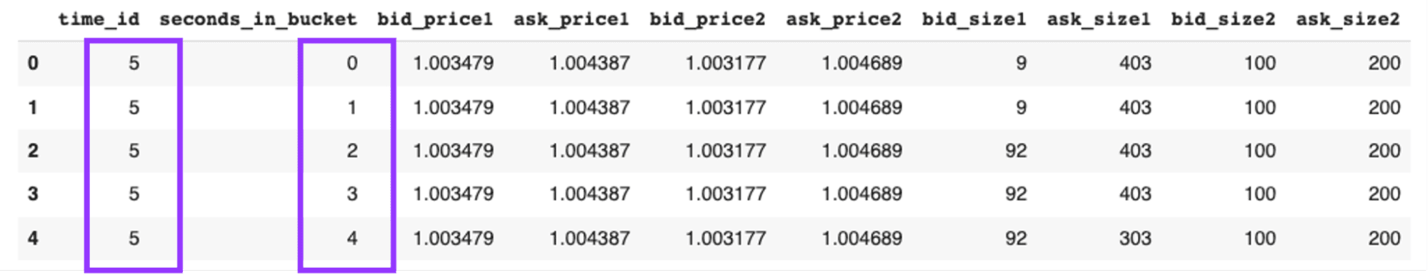
Exhibit-10: Forward Filling The Order Data (Image by Author)
Unlike the data in Exhibit 7, the forward-filled data in Exhibit 10 has all 600 seconds in the time bucket “5” as from 0 to 599, inclusive. We do the same operation on the trade data as well.
2. Merging Data Frames
We have two datasets, order and trade, and both are forward-filled. Both datasets are represented in Pandas and cuDF frameworks. Next, we will merge order and trade datasets on time_id and seconds_in_buckets.
def merge_dataframes(df1, df2, dframe=0):

   print("MERGING DATA FRAMES", "\n")

   if dframe == 0:
     df_type = "Pandas"
   else:
     df_type = "cuDF"

   # Merge dataframes
   print(f"Merging {df_type} dataframes..", "\n")
   start = time.time()
   df = df1.merge(df2, how="left", on=["time_id", "seconds_in_bucket"], sort=True)
   end = time.time()
   elapsed_time = round(end-start, 3)
   print(f"For {df_type} dataframes: \n start time: {start} \n end time: {end} \n elapsed time: {elapsed_time} \n")

   return df, elapsed_time
cuDF will execute the following command:
# Merge cuDF order and trade dataframes
df_cudf, cudf_merge_time = merge_dataframes(expanded_df_cudf_order, expanded_df_cudf_trade, dframe=1)
display(df_cudf.head())
expanded_df_cudf_trade is the forward-filled trade data and is obtained the same way as expanded_df_pd_order or expanded_df_cudf_order. Merge operation will create a combined data frame as shown below:
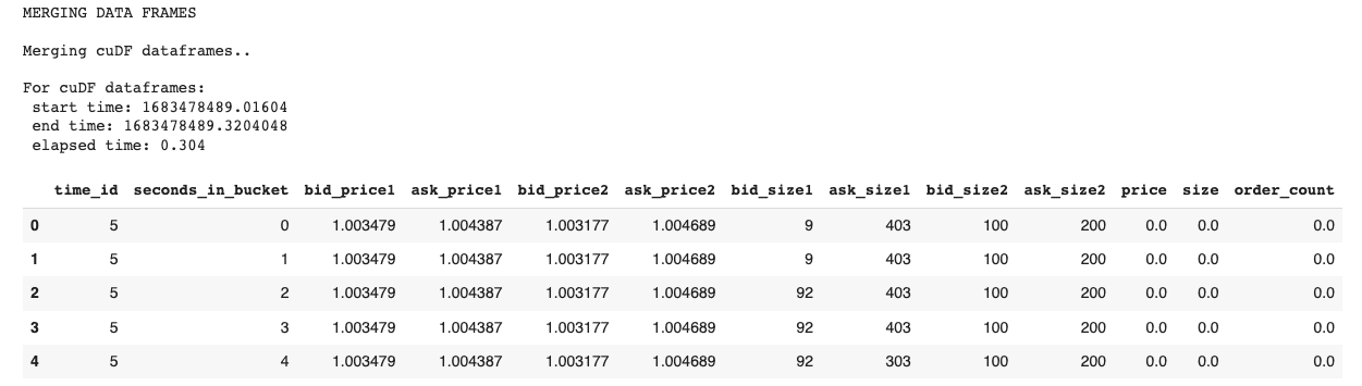
Exhibit-11: Merging Data Frames (Image by Author)
All columns of the two datasets are combined into one. Merging operation is repeated for the Pandas data frames too.

Image by pikisuperstar on Freepik
3. Changing Dtype
We want to change the data type of some columns to reduce memory space and increase computation speed.
# Make dtype changes
def change_dtype(df, dframe=0):

   print("CHANGING DTYPES", "\n")

   convert_dict = {"time_id": "int16",
                   "seconds_in_bucket": "int16",
                   "bid_size1": "int16",
                   "ask_size1": "int16",
                   "bid_size2": "int16",
                   "ask_size2": "int16",
                   "size": "int16",
                   "order_count": "int16"
                   }

   df = df.astype(convert_dict)

   return df, dframe
When we execute the below command,
# Make dtype changes for cuDF data frame
df_cudf, _ = change_dtype(df_cudf)
display(df_cudf.info())
we get the following output:

Exhibit-12: Changing Dtype (Image by Author)
The data in Exhibit 12 would use more memory space if no data type conversion took place. It still has 78.9 MB but, that was after the forward-fill and merge operations, which resulted in 13 columns and 2.3 million entries.
We fulfill every feature engineering task for both Pandas DF and cuDF. Here, we just showed the one for cuDF as an example.
4. Getting Unique Time Ids
We will use the unique method to extract the time_ids in this section.
# Get unique values in time_id column and put them in a list
def get_unique_timeids(df, dframe=0):

   global time_ids

   print("GETTING UNIQUE VALUES", "\n")

   # Get unique time_ids
   if dframe == 0:
     print(f"Getting sorted unique time_ids from Pandas dataframe..", "\n")
     start = time.time()
     time_ids = sorted(df['time_id'].unique().tolist())
     end = time.time()
     elapsed_time = round(end-start, 3)
     print(f"Unique time_ids from Pandas dataframe: \n start time: {start} \n end time: {end} \n elapsed time: {elapsed_time} \n")

   else:
     print(f"Getting sorted unique time_ids from cuDF dataframe..", "\n")
     start = time.time()
     time_ids = sorted(df['time_id'].unique().to_arrow().to_pylist())
     end = time.time()
     elapsed_time = round(end-start, 3)
     print(f"Unique time_ids from cuDF dataframe: \n start time: {start} \n end time: {end} \n elapsed time: {elapsed_time} \n")

   print(f"{len(time_ids)} time buckets: \n {time_ids[:10]}...")
   print("\n")

   return df, time_ids
The above code will get the unique time_ids from Pandas DF and cuDF.
# Get time_ids from cuDF dataframe
time_ids = get_unique_timeids(df_cudf_order, dframe=1)
The output of the cuDF looks like this:
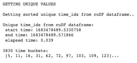
Exhibit-13: Getting Unique Time Ids (Image by Author)
5. Checking Null Values
Then, we will check the null values in data frames.
# Check df null values
def check_null_values(df, dframe=0):

   print("CHECKING NULL VALUES", "\n")

   print("Checking dataframe null values..", "\n")
   display(df.isna().values.any())
   display(df.isnull().sum())

   return df, dframe
Checking null values example in cuDF:
# Check null values for cuDF dataframe
df_cudf, _ = check_null_values(df_cudf, dframe=0)
And the output is:
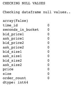
Exhibit-14: Checking Null Values (Image by Author)
6. Adding a Column
We want to create more features, so add a few columns.
# Add columns
def add_column(df, dframe=0):

   print("ADDING COLUMNS", "\n")

   # Calculate WAPs
   df['wap1'] = (df['bid_price1'] * df['ask_size1'] + df['ask_price1'] * df['bid_size1']) / (df['bid_size1'] + df['ask_size1'])
   df['wap2'] = (df['bid_price2'] * df['ask_size2'] + df['ask_price2'] * df['bid_size2']) / (df['bid_size2'] + df['ask_size2'])

   # Calculate order volumes
   df['bid1_volume'] = df['bid_price1'] * df['bid_size1']
   df['bid2_volume'] = df['bid_price2'] * df['bid_size2']
   df['ask1_volume'] = df['ask_price1'] * df['ask_size1']
   df['ask2_volume'] = df['ask_price2'] * df['ask_size2']

   # Calculate volume imbalance
   df['imbalance'] = np.absolute((df['ask_size1'] + df['ask_size2']) - (df['bid_size1'] + df['bid_size2']))

   # Calculate trade volume imbalance
   df['volume_imbalance'] = np.absolute((df['bid_price1'] * df['bid_size1']) - (df['ask_price1'] * df['ask_size1']))

   return df, dframe
That will create new features such as weighted average price (wap1 and wap2), order volume, and volume imbalance. In total, eight columns will be added to the data frames by executing the following:
# Add a column in cuDF dataframe
df_cudf, _ = add_column(df_cudf)
display(df_cudf.head())
It will hence give us:
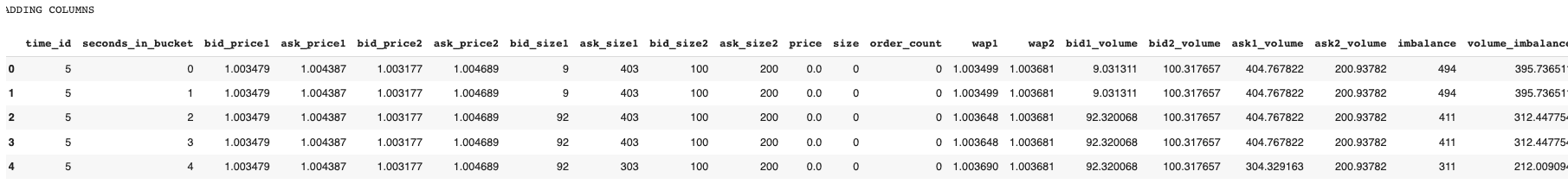
Exhibit-15: Adding Columns And Features (Image by Author)
7. Dropping a Column
We decide to get rid of two features, wap1 and wap2, by dropping their columns:
# Drop columns
def drop_column(df, dframe=0):

   print("DROPPING COLUMNS", "\n")

   df.drop(columns=['wap1', 'wap2'], inplace=True)

   return df, dframe
Implementation of dropping columns is:
# Add a column in cuDF dataframe
df_cudf, _ = drop_column(df_cudf)
display(df_cudf.head())
That leaves us with the data frames that wap1, and wap2 columns are gone!
8. Calculating Statistics by Group
Next, we calculate the mean, median, maximum, minimum, standard deviation, and the sum of some features by time_id. For this, we will use groupby and agg methods.
# Calculate statistics by selected features
def calc_agg_stats(df, dframe=0):

   print("CALCULATING STATISTICS", "\n")

   # Statistical calculations to be made
   operations = ["mean", "median", "max", "min", "std", "sum"]

   # Features for which statistical calculations will be made
   features_list = ["bid1_volume", "bid2_volume", "ask1_volume", "ask2_volume"]

   # Create a dictionary to store feature-calculation pairs
   stats_dict = defaultdict(list)
   for feature in features_list:
       stats_dict[feature].extend(operations)

   # Calculate aggregate statistics
   df_stats = df.groupby('time_id', as_index=False, sort=True).agg(stats_dict)

   return df, df_stats
We create a list named features_list to specify the features that the mathematical calculations will be performed.
# Calculate statistics by selected features in cuDF dataframe
_, df_cudf_stats = calc_agg_stats(df_cudf)
display(df_cudf_stats.head())
In return, we get the following output:
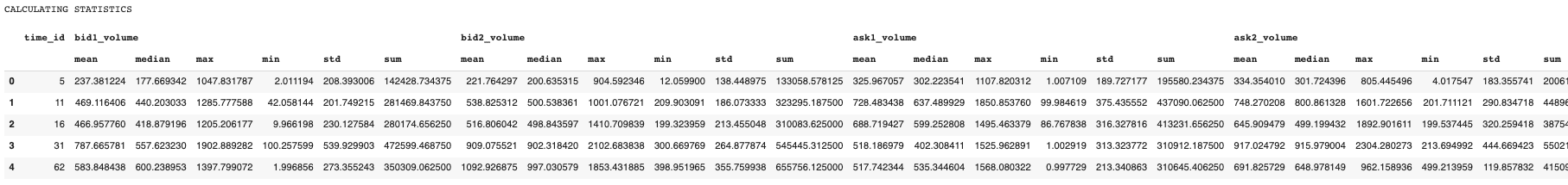
Exhibit-16: Calculating Statistics (Image by Author)
The returned table is a new data frame. We should merge it with the original one (df_cudf). We will accomplish it through Pandas:
# Merge data frame with stats
def merge_dataframes_2(df, dframe=0):

   if dframe == 0:
     df = df.merge(df_pd_stats, how="left", on="time_id", sort=True)

   else:
     df = df.to_pandas()
     df = df.merge(df_pd_stats, how="left", on="time_id", sort=True)
     df = cudf.DataFrame.from_pandas(df)

   return df, dframe


# Merge cuDF data frames
df_cudf, _ = merge_dataframes_2(df_cudf, dframe=1)
display(df_cudf.head())
The above snippet will put df_pd_stats and df_pd in one data frame and save it as df_cudf.
As usual, we repeat the same task for Pandas.
The next step is to calculate the correlation between two columns:
# Calculate correlation between two selected features
def calc_corr(df, dframe=0):

 correlation = df[["bid1_volume", "ask1_volume"]].corr()
 print(f"Correlation between 'bid1_volume' and 'ask1_volume' is {correlation} \n")

 return df, correlation
This code
# Calculate correlation in cuDF dataframe
_ = calc_corr(df_cudf)
will return the following output:
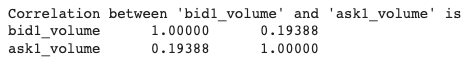
Exhibit-17: Calculating Correlation Between Two Features (Image by Author)
9. Renaming Columns
To remove any confusion, we should rename two of our columns.
# Rename columns
def rename_cols(df, dframe=0):

   print("RENAMING COLUMNS", "\n")

   df = df.rename(columns={"imbalance": "volume_imbalance", "volume_imbalance": "trade_volume_imbalance"})

   return df, dframe
Columns imbalance and volume_imbalance will be renamed as volume_imbalance and trade_volume_imbalance, respectively.
10. Binning a Column
Another data manipulation we want to make is to bin the bid1_volume and store the bins in a new column.
# Bin a selected column
def bin_col(df, dframe=0):

   print("BINNING A COLUMN", "\n")

   if dframe == 0:
     df['bid1_volume_cut'] = pd.cut(df["bid1_volume"], bins=5, labels=["very high", "high", "average", "low", "very low"], ordered=True)

   else:
     df['bid1_volume_cut'] = cudf.cut(df["bid1_volume"], bins=5, labels=["very high", "high", "average", "low", "very low"], ordered=True)

   return df, dframe
By running the lines
# Bin a selected column in cuDF dataframe
df_cudf, _ = bin_col(df_cudf, dframe=1)
display(df_cudf.head())
we’ll get a data frame as the output, which we may see a part of it as shown below:
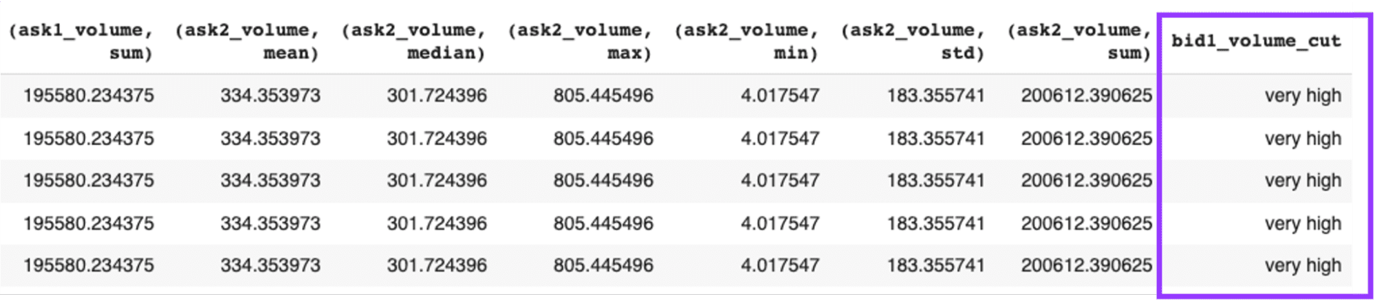
Exhibit-18: Binning A Column (Image by Author)
11. Displaying Data Frames
After feature engineering steps are completed, we can present the data frames. This section contains three operations: displaying the data frame, getting information about it, and describing it.
# Display data frame
def display_df(df, dframe=0):

   print("DISPLAYING DATA FRAMES", "\n")

   display(df.head())
   print("\n")

   return df, dframe


# Display dataframe info
def display_info(df, dframe=0):

   print("DISPLAYING DATA FRAME INFO", "\n")

   display(df.info())
   print("\n")

   return df, dframe


# Display dataframe info
def describe_df(df, dframe=0):

   print("DESCRIBING DATA FRAMES", "\n")

   display(df.describe())
   print("\n")

   return df, dframe
The following code will finalize these three tasks:
# Display cuDF dataframe and info
_, _ = display_df(df_cudf, dframe=1)
_, _ = display_info(df_cudf, dframe=1)
_, _ = describe_df(df_cudf, dframe=1)
We are done with feature engineering.
Single-Run Execution
In summary, our feature engineering efforts have focused on the following tasks:
- Loading data frames
- Merging data frames
- Changing data type
- Getting unique time_ids.
- Checking null values
- Adding columns
- Dropping columns
- Calculating statistics
- Calculating a correlation
- Renaming columns
- Binning a column
- Displaying data frames
- Displaying data information
- Describing data frames
It was all 13 tasks, but we mentioned “Calculating a correlation” as a separate entity here. Now, we want to run these tasks sequentially in a single run, as shown below:
def run_and_report():

   # Create a dictionary to store elapsed times
   time_dict = defaultdict(list)

   # List operations to be performed
   labels = ["changing_dtype",
             "getting_unique_timeids",
             "checking_null_values",
             "adding_column",
             "dropping_column",
             "calculating_agg_stats",
             "merging_dataframes",
             "renaming_columns",
             "binning_col",
             "calculating_corr",
             "displaying_dfs",
             "displaying_info",
             "describing_dfs"]

   # Load pandas order dataframe and calculate time
   df_pd_order, pd_order_loading_time = load_dataframe(order_files, dframe=0)
   print("-"*150, "\n")

   # Load cuDF book dataframe and calculate time
   df_cudf_order, cudf_order_loading_time = load_dataframe(order_files, dframe=1)
   print("-"*150, "\n")

   # Load pandas trade dataframe and calculate time
   df_pd_trade, pd_trade_loading_time = load_dataframe(trade_files, dframe=0)
   print("-"*150, "\n")

   # Load cuDF trade dataframe and calculate time
   df_cudf_trade, cudf_trade_loading_time = load_dataframe(trade_files, dframe=1)
   print("-"*150, "\n")

   # Get time_ids from Pandas data frame
   _, time_ids = get_unique_timeids(df_pd_order, dframe=0)
   print("-"*150, "\n")

   # Get time_ids from cuDF dataframe
   _, time_ids = get_unique_timeids(df_cudf_order, dframe=1)
   print("-"*150, "\n")

   # Store loading times
   time_dict["loading_dfs"].extend([pd_order_loading_time, cudf_order_loading_time])

   # Forward fill order dataframes
   expanded_df_pd_order, expanded_df_cudf_order = ffill(df_pd_order, df_name="order")

   # Forward fill trade dataframes
   expanded_df_pd_trade, expanded_df_cudf_trade = ffill(df_pd_trade, df_name="trade")

   # Merge pandas order and trade dataframes
   df_pd, pd_merge_time = merge_dataframes(expanded_df_pd_order, expanded_df_pd_trade, dframe=0)
   print("-"*150, "\n")

   # Merge pandas order and trade dataframes
   df_cudf, cudf_merge_time = merge_dataframes(expanded_df_cudf_order, expanded_df_cudf_trade, dframe=1)
   print("-"*150, "\n")

   # Store merge times
   time_dict["merging_dfs"].extend([pd_merge_time, cudf_merge_time])

   # Apply functions
   functions = [change_dtype,
                get_unique_timeids,
                check_null_values,
                add_column,
                drop_column,
                calc_agg_stats,
                merge_dataframes_2,
                rename_cols,
                bin_col,
                calc_corr,
                display_df,
                display_info,
                describe_df]

   for label, function in enumerate(functions):

     # Function for pandas
     start_pd = time.time()
     df_pd, x = function(df_pd, dframe=0)
     end_pd = time.time()
     elapsed_time_for_pd = round(end_pd-start_pd, 3)
     print(f"For pandas dataframe: \n start time: {start_pd} \n end time: {end_pd} \n elapsed time: {elapsed_time_for_pd} \n")

     # Function for cuDF
     start_cudf = time.time()
     df_cudf, x = function(df_cudf, dframe=1)
     end_cudf = time.time()
     elapsed_time_for_cudf = round(end_cudf-start_cudf, 3)
     print(f"For cuDF dataframe: \n start time: {start_cudf} \n end time: {end_cudf} \n elapsed time: {elapsed_time_for_cudf} \n")
     print("-"*150, "\n")

     # Store elapsed times
     time_dict[labels[label]].extend([elapsed_time_for_pd, elapsed_time_for_cudf])

   # Delete the unsolicited time duration
   del time_dict["merging_dataframes"]
   labels.remove("merging_dataframes")
   labels.insert(0, "merging_dfs")
   labels.insert(0, "loading_dfs")

   print(time_dict)

   return time_dict, labels, df_pd, df_cudf
The run_and_report function will give the same outputs as before but in a full report by a single execution command. It will execute the 14 tasks on both Pandas and cuDF and record the times they take for both data frames.
time_dict, labels, df_pd, df_cudf = run_and_report()
We may have to run multiple cycles to see the relative performance of both data libraries more boldly.
Final Evaluation
If we run the run_and_report multiple times, such as in rounds, we can get a better sense of the difference in performance between Pandas and cuDF. So, we set rounds as 30. Then, we record all time durations for every operation, round, and data library and finally evaluate the results:
def calc_exec_times():

   exec_times_by_round = {}

   # Calculate execution times of operations in each round
   for round_no in range(1, ROUNDS+1):
     # cycle_no += 1
     time_dict, labels, df_pd, df_cudf = run_and_report()
     exec_times_by_round[round_no] = time_dict

   print("exec_times_by_round: ", exec_times_by_round)

   # Get durations by operation for each data frame
   pd_summary, cudf_summary = get_statistics(exec_times_by_round, labels)

   # Get durations by rounds for each data frame
   round_total = get_total(exec_times_by_round)
   print("\n"*3)

   # Plot durations
   plt.style.use('dark_background')
   X_axis = np.arange(len(labels))

   # Plot average duration of operation
   plot_avg_by_df(pd_summary, cudf_summary, labels, X_axis)
   print("\n"*3)

   # Plot total and difference in duration by operation
   plot_diff_by_df(pd_summary, cudf_summary, labels)
   print("\n"*3)

   # Plot total and difference in duration by round
   plot_total_by_df(round_total)
   print("\n"*3)
The calc_exec_times function executes a few tasks. It first calls get_statistics to get the “average and total time durations by operation” for each data library over 30 rounds.
def get_statistics(exec_times_by_round, labels):

   # Separate and store duration statistics by data frame
   pd_performance = defaultdict(list)
   cudf_performance = defaultdict(list)

   # Get and store durations for each operation by data frame
   for label in labels:
     for key, values in exec_times_by_round.items():

       pd_performance[label].append(values[label][0])
       cudf_performance[label].append(values[label][1])

   print("pd_performance: ", pd_performance)
   print("cudf_performance: ", cudf_performance)

   # Compute average and total durations for each operation by data frame
   pd_summary = {key: [round(sum(value), 3), round(np.average(value), 3)] for key, value in pd_performance.items()}
   cudf_summary = {key: [round(sum(value), 3), round(np.average(value), 3)] for key, value in cudf_performance.items()}

   print("pd_summary: ", pd_summary)
   print("cudf_summary: ", cudf_summary)

   return pd_summary, cudf_summary
Next, it computes the “total duration by round” for each data framework.
def get_total(exec_times_by_round):

   def get_round_total(stat_list):

     # Get total duration by round for each data frame
     pd_round_total = round(sum([x[0] for x in stat_list]), 3)
     cudf_round_total = round(sum([x[1] for x in stat_list]), 3)

     return pd_round_total, cudf_round_total

   # Collect total durations by round
   for key, value in exec_times_by_round.items():
     round_total = {key: get_round_total(list(value.values())) for key, value in exec_times_by_round.items()}

   print("round_total", round_total)

   return round_total
Lastly, it plots the results. Here, the first plot is for the “average time duration by operation” for both libraries.
def plot_avg_by_df(pd_summary, cudf_summary, labels, X_axis):

   # Figure size
   fig = plt.subplots(figsize =(10, 4))

   # Average duration by operation for each data frame
   pd_avg = [value[1] for key, value in pd_summary.items()]
   cudf_avg = [value[1] for key, value in cudf_summary.items()]

   plt.bar(X_axis - 0.2, pd_avg, 0.4, color = '#5A5AAF', label = 'pandas', align='center')
   plt.bar(X_axis + 0.2, cudf_avg, 0.4, color = '#C8C8FF', label = 'cuDF', align='center')

   plt.xticks(X_axis, labels, fontsize=9, rotation=90)
   plt.yticks(fontsize=9)
   plt.xlabel("Operations", fontsize=10)
   plt.ylabel("Average Duration in Seconds", fontsize=10)
   plt.grid(axis='y', color="#E4E4E4", alpha=0.5)
   plt.title("Average Duration of Operation by Data Frame", fontsize=12)
   plt.legend()
   plt.show()
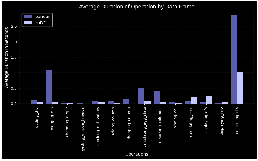
Exhibit-19: Average Duration By Operation For Pandas Data Frame And cuDF (Image by Author)
The second plot is for the “total duration by operation,” which shows the total time each task took over all 30 rounds.
def plot_diff_by_df(pd_summary, cudf_summary, labels):

   # Figure size
   fig = plt.subplots(figsize =(12, 6))

   # Total duration by operation for each data frame
   pd_total = [value[0] for key, value in pd_summary.items()]
   cudf_total = [value[0] for key, value in cudf_summary.items()]

   # Difference of total duration by operation for each data frame
   diff = [x[0]-x[1] for x in zip(pd_total, cudf_total)]

   # Set width of bar
   barWidth = 0.25

   # Set position of bar on X axis
   br1 = np.arange(len(labels))
   br2 = [x + barWidth for x in br1]
   br3 = [x + barWidth for x in br2]

   plt.bar(br1, pd_total, barWidth, color = '#5A5AAF', label = 'pandas', align='center')
   plt.bar(br2, cudf_total, barWidth, color = '#C8C8FF', label = 'cuDF', align='center')
   plt.bar(br3, diff, barWidth, color = '#AA1E1E', label = 'difference', align='center')

   plt.xticks([r + barWidth for r in range(len(labels))], labels, fontsize=9, rotation=90)
   plt.yticks(fontsize=9)
   plt.xlabel("Operations", fontsize=10)
   plt.ylabel("Total Duration in Seconds", fontsize=10)
   plt.grid(axis='y', color="#E4E4E4", alpha=0.5)
   plt.title("Total Duration of Operation by Data Frame", fontsize=12)
   plt.legend()
   plt.show()
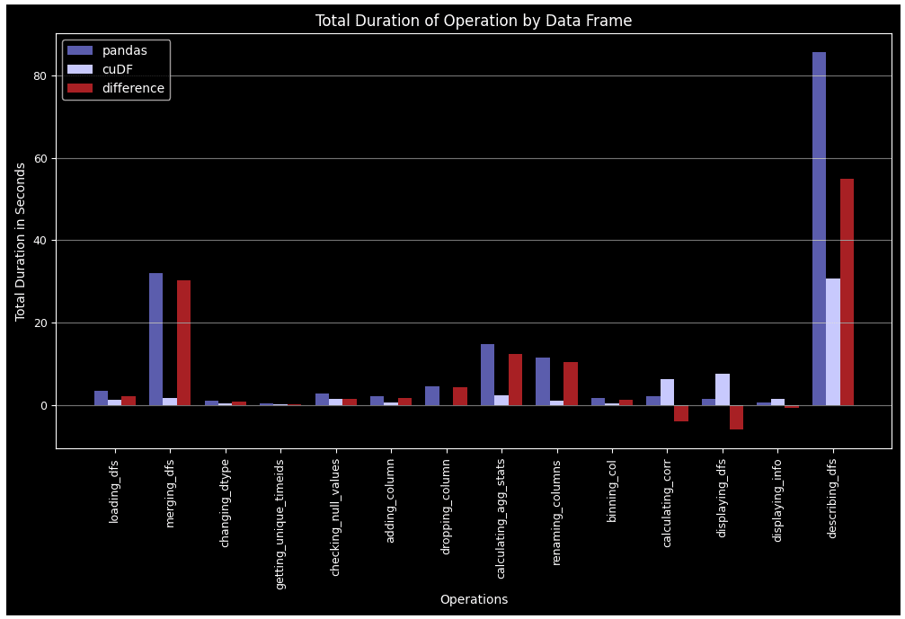
Exhibit-20: Total Duration By Operation Over 30 Rounds For Pandas Data Frame And cuDF (Image by Author)
The final plot is “total duration by round,” which shows the total time all operations took together for each round.
def plot_total_by_df(round_total):

    # Figure size
   fig = plt.subplots(figsize =(10, 6))

   X_axis = np.arange(1, ROUNDS+1)

   # Total duration by round for each data frame
   pd_round_total = [value[0] for key, value in round_total.items()]
   cudf_round_total = [value[1] for key, value in round_total.items()]

   # Difference of total duration by round for each data frame
   diff = [x[0]-x[1] for x in zip(pd_round_total, cudf_round_total)]

   plt.plot(X_axis, pd_round_total, linestyle="-", linewidth=3, color = '#5A5AAF', label = "pandas")
   plt.plot(X_axis, cudf_round_total, linestyle="-", linewidth=3, color = '#B0B05A', label = "cuDF")
   plt.plot(X_axis, diff, linestyle="--", linewidth=3, color = '#AA1E1E', label = "difference")

   plt.xticks(X_axis, fontsize=9)
   plt.yticks(fontsize=9)
   plt.xlabel("Rounds", fontsize=10)
   plt.ylabel("Total Duration in Seconds", fontsize=10)
   plt.grid(axis='y', color="#E4E4E4", alpha=0.5)
   plt.title("Total Duration by Round", fontsize=12)
   plt.legend()
   plt.show()
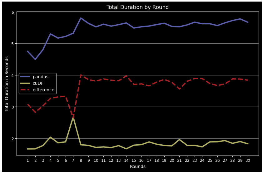
Exhibit-21: Total Duration Of All Operations For Each Round For Pandas Data Frame And cuDF (Image by Author)
Even though we haven’t covered every feature engineering task fulfilled on the dataset, they are the same as or similar to the ones we showed here. By explaining 14 operations individually, we tried to document the relative performance of Pandas data frame and cuDF, and enable reproducibility.
In all cases except for correlation calculation and data frame display, cuDF surpasses Pandas. This performance lead becomes more remarkable in complex tasks such as groupby, merge, agg, and describe. Another point is Pandas DF gets tired over time when more rounds come over, while cuDF follows a more stable pattern.
Recall that we have reviewed only one stock as an example. If we process all 112 stocks, we may expect a larger performance gap in favor of cuDF. If the stock's population goes up to the hundreds, cuDF’s performance can even be more dramatic. In the case of big data, where the execution of parallel tasks is possible, a distributed framework such as Dask-cuDF, which extends parallel computing to cuDF GPU DataFrames, can be the right tool.
References
[1] RAPIDS Definition, https://www.heavy.ai/technical-glossary/rapids
[2] 10 Minutes to cuDF and Dask-cuDF, https://docs.rapids.ai/api/cudf/stable/user_guide/10min/
[3] Optiver Realized Volatility Prediction, https://www.kaggle.com/competitions/optiver-realized-volatility-prediction/data
[4] Forward filling book data, https://www.kaggle.com/competitions/optiver-realized-volatility-prediction/discussion/251277
Hasan Serdar Altan is Data scientist and AWS Cloud Architect Associate.