Leveraging XGBoost for Time-Series Forecasting
Enabling the powerful algorithm to forecast from your data.
XGBoost (eXtreme Gradient Boosting) is an open-source algorithm that implements gradient-boosting trees with additional improvement for better performance and speed. The algorithm's quick ability to make accurate predictions makes the model a go-to model for many competitions, such as the Kaggle competition.
The common cases for the XGBoost applications are for classification prediction, such as fraud detection, or regression prediction, such as house pricing prediction. However, extending the XGBoost algorithm to forecast time-series data is also possible. How is it works? Let’s explore this further.
Time-Series Forecasting
Forecasting in data science and machine learning is a technique used to predict future numerical values based on historical data collected over time, either in regular or irregular intervals.
Unlike common machine learning training data where each observation is independent of the other, data for time-series forecasts must be in successive order and related to each data point. For example, time-series data could include monthly stock, weekly weather, daily sales, etc.
Let’s look at the example time-series data Daily Climate data from Kaggle.
import pandas as pd

train = pd.read_csv('DailyDelhiClimateTrain.csv')
test = pd.read_csv('DailyDelhiClimateTest.csv')

train.head()
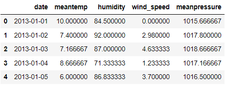
If we look at the dataframe above, every feature is recorded daily. The date column signifies when the data is observed, and each observation is related.
Time-Series forecast often incorporate trend, seasonal, and other patterns from the data to create forecasting. One easy way to look at the pattern is by visualizing them. For example, I would visualize the mean temperature data from our example dataset.
train["date"] = pd.to_datetime(train["date"])
test["date"] = pd.to_datetime(test["date"])

train = train.set_index("date")
test = test.set_index("date")

train["meantemp"].plot(style="k", figsize=(10, 5), label="train")
test["meantemp"].plot(style="b", figsize=(10, 5), label="test")
plt.title("Mean Temperature Dehli Data")
plt.legend()
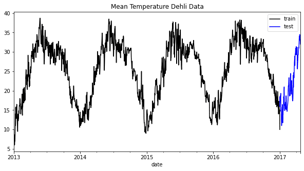
It’s easy for us to see in the graph above that each year has a common seasonality pattern. By incorporating this information, we can understand how our data work and decide which model might suit our forecast model.
Typical forecast models include ARIMA, Vector AutoRegression, Exponential Smoothing, and Prophet. However, we can also utilize XGBoost to provide the forecasting.
XGBoost Forecasting
Before preparing to forecast using XGBoost, we must install the package first.
pip install xgboost
After the installation, we would prepare the data for our model training. In theory, XGBoost Forecasting would implement the Regression model based on the singular or multiple features to predict future numerical values. That is why the data training must also be in the numerical values. Also, to incorporate the motion of time within our XGBoost model, we would transform the time data into multiple numerical features.
Let’s start by creating a function to create the numerical features from the date.
def create_time_feature(df):
    df['dayofmonth'] = df['date'].dt.day
    df['dayofweek'] = df['date'].dt.dayofweek
    df['quarter'] = df['date'].dt.quarter
    df['month'] = df['date'].dt.month
    df['year'] = df['date'].dt.year
    df['dayofyear'] = df['date'].dt.dayofyear
    df['weekofyear'] = df['date'].dt.weekofyear
    return df
Next, we would apply this function to the training and test data.
train = create_time_feature(train)
test = create_time_feature(test)

train.head()
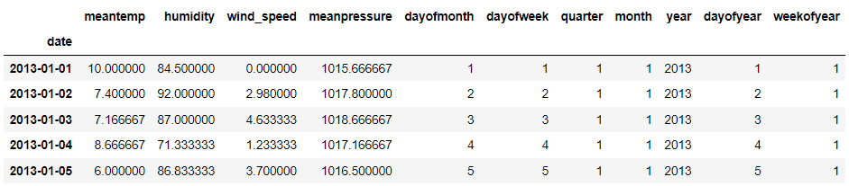
The required information is now all available. Next, we would define what we want to predict. In this example, we would forecast the mean temperature and make the training data based on the data above.
X_train = train.drop('meantemp', axis =1)
y_train = train['meantemp']

X_test = test.drop('meantemp', axis =1)
y_test = test['meantemp']
I would still use the other information, such as humidity, to show that XGBoost can also forecast values using multivariate approaches. However, in practice, we only incorporate data that we know exists when we try to forecast.
Let’s start the training process by fitting the data into the model. For the current example, we would not do much hyperparameter optimization other than the number of trees.
import xgboost as xgb

reg = xgb.XGBRegressor(n_estimators=1000)
reg.fit(X_train, y_train, verbose = False)
After the training process, let’s see the feature importance of the model.
xgb.plot_importance(reg)
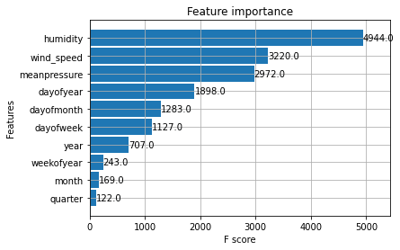
The three initial features are not surprisingly helpful for forecasting, but the time features also contribute to the prediction. Let’s try to have the prediction on the test data and visualize them.
test['meantemp_Prediction'] = reg.predict(X_test)

train['meantemp'].plot(style='k', figsize=(10,5), label = 'train')
test['meantemp'].plot(style='b', figsize=(10,5), label = 'test')
test['meantemp_Prediction'].plot(style='r', figsize=(10,5), label = 'prediction')
plt.title('Mean Temperature Dehli Data')
plt.legend()
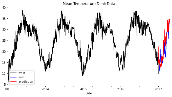
As we can see from the graph above, the prediction might seem slightly off but still follow the overall trend. Let’s try to evaluate the model based on the error metrics.
from sklearn.metrics import mean_squared_error, mean_absolute_error, mean_absolute_percentage_error

print('RMSE: ', round(mean_squared_error(y_true=test['meantemp'],y_pred=test['meantemp_Prediction']),3))
print('MAE: ', round(mean_absolute_error(y_true=test['meantemp'],y_pred=test['meantemp_Prediction']),3))
print('MAPE: ', round(mean_absolute_percentage_error(y_true=test['meantemp'],y_pred=test['meantemp_Prediction']),3))
RMSE: 11.514
MAE: 2.655
MAPE: 0.133
The result shows that our prediction may have an error of around 13%, and the RMSE also shows a slight error in the forecast. The model can be improved using hyperparameter optimization, but we have learned how XGBoost can be used for the forecast.
Conclusion
XGBoost is an open-source algorithm often used for many data science cases and in the Kaggle competition. Often the use cases are common classification cases such as fraud detection or regression cases such as house price prediction, but XGBoost can also be extended into time-series forecasting. By using the XGBoost Regressor, we can create a model that can predict future numerical values.
Cornellius Yudha Wijaya is a data science assistant manager and data writer. While working full-time at Allianz Indonesia, he loves to share Python and Data tips via social media and writing media.