Avoid These Mistakes with Time Series Forecasting
A few checks to make before training a Machine Learning model on data that could be random.
By Roman Orac, Senior Data Scientist

Photo by Photoholgic on Unsplash
Time series forecasting is a subfield of Data Science, which deals with forecasting the spread of COVID, forecasting the prices of stocks, forecasting the daily consumption of electricity… we could go on and on.
Data Science is a wide field of study and there aren’t many “Jack of all trades”
The Data Science field is a wide field of study. Many Data Scientists work their whole careers with non-sequential data (classical classification and regression Machine Learning) and they never train a time series forecasting model in their professional career.
This is to be expected because of the rapid growth of the Data Science field. It’s harder and harder to keep up with all the subfields.
Data Scientists who plan to pivot into the world of time series can prepare for a fun ride because working with this kind of data requires different, specialized approaches.
In this article, we’ll go through a few common Time Series forecasting pitfalls that are easy to fall into. I based the examples on financial stock data but the approaches can be used with any other time-series data.
By reading this article, you’ll learn:
- How to download financial time series data with pandas
- How to find peaks and troughs in a time series signal
- What is (and how to use) autocorrelation plot
- How to check if a time series has any statistically significant signal
Jack of all trades, master of none
We simply need to collect the data

Photo by Hans Eiskonen on Unsplash
One fallacy (and a doomed project from the start) is when software engineers think that they can simply collect the stock market data and then put it in a Deep Neural Network to find profitable patterns.
Deep Neural Net will find profitable patterns automatically, right?
Don’t get me wrong, having data is useful, but the hardest part comes with the modeling.
There are Data Service sites, like EOD Historical Data, which offer all kinds of financial data with a free plan. It makes more sense to try to identify profitable patterns first as you can download historical data with single pandas command.
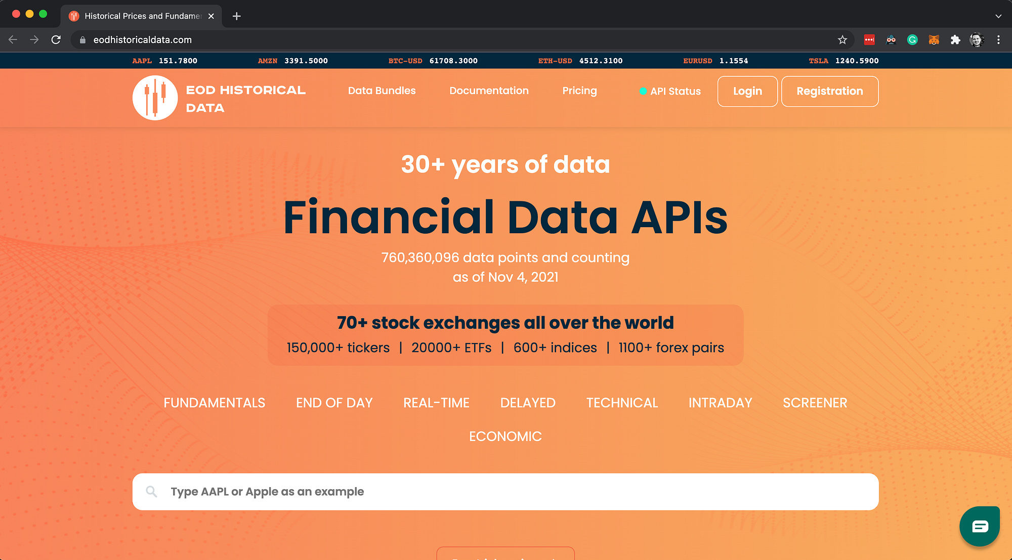
EOD Historical Data offers all kinds of financial data with a free plan (screenshot made by author)
What’s that pandas command to download the data?
Let’s look at the example below, in which I download daily Apple stock prices from 1st January 2018 and onward:
import pandas as pdstock = "AAPL.US"
from_date = "2018-01-01"
to_date = "2021-10-29"
period = "d"eon_url = f"https://eodhistoricaldata.com/api/eod/{stock}?api_token=OeAFFmMliFG5orCUuwAKQ8l4WWFQ67YX&from={from_date}&to={to_date}&period={period}&fmt=json"df = pd.read_json(eon_url)
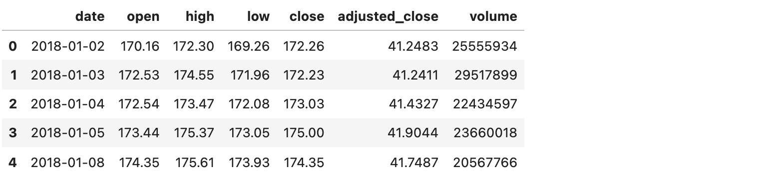
Daily Apple stock prices from 1st January 2018 and onwards (image by author)
We can then visualize the adjusted close prices of Apple stock and prices distribution with:
fig, axes = plt.subplots(nrows=1, ncols=2, figsize=(14, 7))col = "adjusted_close"
df.plot(x="date", y=col, ax=axes[0])
df[col].hist(ax=axes[1])
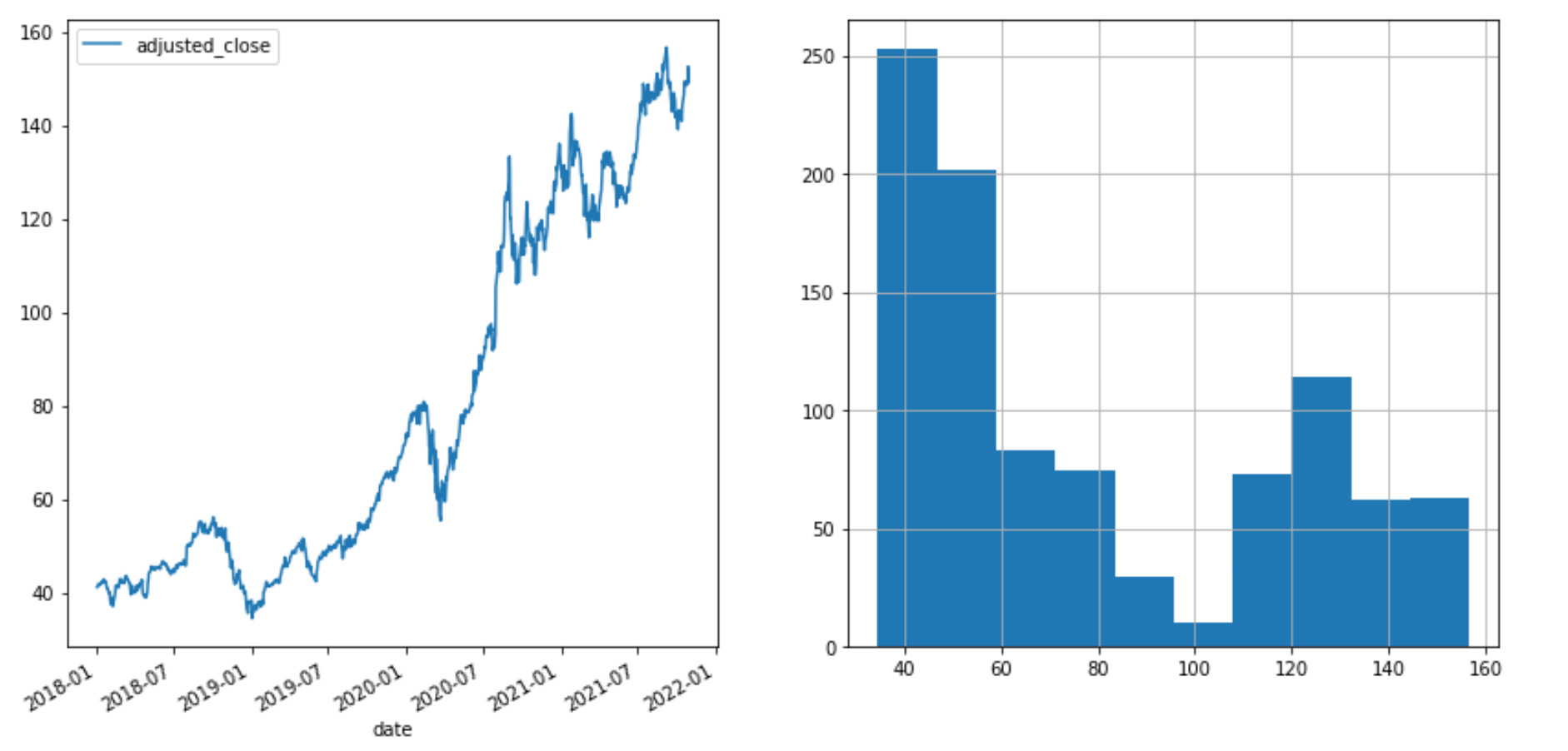
Adjusted close prices and distribution of Apple stock price (image by author)
Finding Peaks and Troughs
Photo by Claudel Rheault on Unsplash
A common way a time series forecasting learning problem is then defined is to find peaks and troughs on the time-series signal, which serve as a target variable for the Machine Learning algorithm.
Let’s first reduce the data size so that we can visualize it easier:
df_sub = df[df["date"] > "2020-01-01"].copy().reset_index(drop=True)
Then finds peaks:
from scipy.signal import find_peakspeaks = find_peaks(df_sub["adjusted_close"])
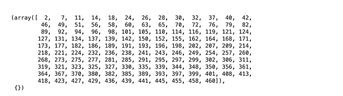
Array with indices of peaks (image by author)
Then find troughs:
troughs = find_peaks(-df_sub["adjusted_close"])
Then we can visualize the
ax = df_sub.plot(x="date", y="adjusted_close", figsize=(14, 7))df_sub.iloc[peaks[0]].plot.scatter(x="date", y="adjusted_close", ax=ax, color="green")df_sub.iloc[troughs[0]].plot.scatter(x="date", y="adjusted_close", ax=ax, color="red")
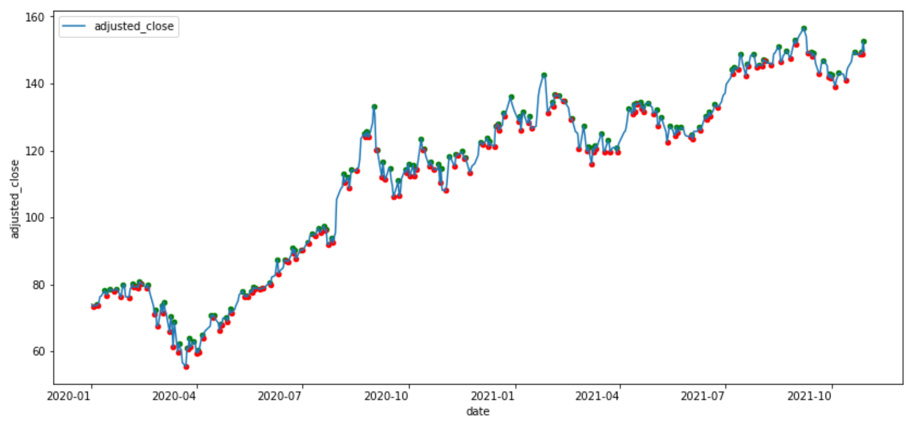
Apple stock time series with peaks and troughs (image by author)
Now that the dataset is marked with entry and exit signals, we just take Neural Net out of the box and sit back and relax, right?
Not exactly!
Technical analysts might point out the lookahead bias in the example above.
Why?
Because the find peaks function worked with the whole signal at once. If we would define decision logic based on lagging indicators on top of it, it would suffer from lookahead bias.
From wikipedia:
In finance, technical analysis is an analysis methodology for forecasting the direction of prices through the study of past market data, primarily price and volume.But that’s a problem only if we would rely on technical analysis.
Let’s go back to Machine Learning.
From a Machine Learning point of view, the definition above is OK if we split the signal into 3 parts. Eg.:
- the first part for training (first 60%)
- the second part for validation (second 10%)
- and last part for out of sample test (last 30%)
The output of the find peaks function is only used for the target and there is no data leak to features.
So what’s wrong with this definition of learning problem?
The one million dollar question we need to answer before applying a Machine Learning algorithm to the data:
Is there any signal in the time series or is it all random noise?
Is there any signal in the time series?
Photo by Clarisse Meyer on Unsplash
Let’s compare randomly generated numbers drawn from the Gaussian distribution with the Apple stock time series.
With the command below I generate 1000 random numbers from Gaussian distribution with zero mean and the standard deviation equal to 1 (aka. normal distribution):
np.random.seed(42)normal_dist = pd.DataFrame(np.random.normal(size=1000), columns=["value"])
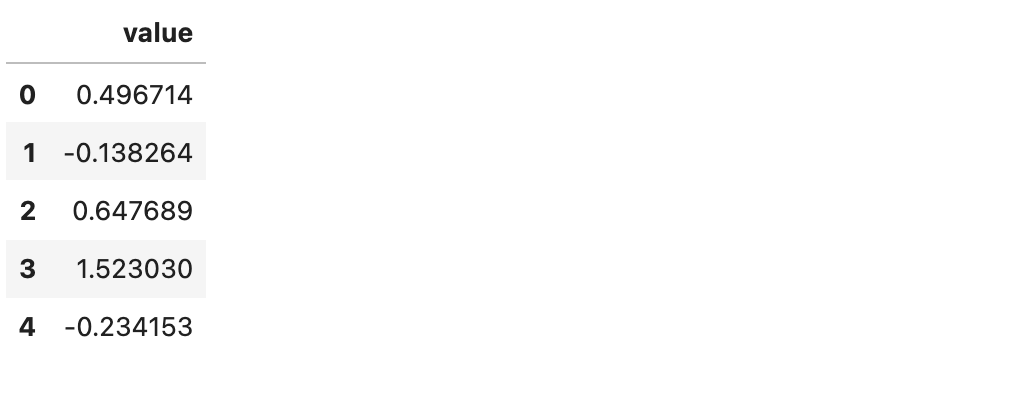
Random numbers were drawn from a normal distribution (image by author)
Now, let’s visualize generated numbers and compare them with Apple stock time series:
fig, axes = plt.subplots(nrows=1, ncols=2, figsize=(14, 7))normal_dist["value"].plot(
    ax=axes[0],
    title="Random samples drawn from a normal (Gaussian) distribution",
)df.plot(x="date", y="adjusted_close", ax=axes[1], title="Apple stock time series")
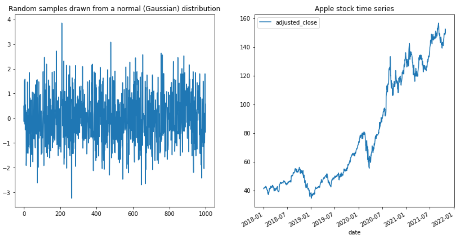
Comparing random samples from Gaussian distribution with Apple stock time series (image by author)
You don’t need to be a scientist to notice that the Apple stock time series has an increasing pattern and Gaussian numbers just randomly jump up and down.
Does the Apple stock time series really have a pattern from which a Machine Learning algorithm can learn a pattern?
Let me take you for a (random) walk
Photo by Jonas Weckschmied on Unsplash
A random walk is a statistical tool, which generates random numbers with -1 and 1 and the next number is dependent on the previous state. This provides some consistency, unlike independent random numbers. The random walk can help us determine if our time series is predictable or not.
Let’s look at the example below.
In the first step, we generate a list of 1000 numbers with randomly selected -1 and 1.
np.random.seed(42)random_walk = pd.DataFrame()
random_walk.loc[:, "random_number"] = np.random.choice([-1, 1], size=1000, replace=True)
Then we cumulative summarize generated random values to add dependence on the previous state:
random_walk.loc[:, "random_walk"] = random_walk["random_number"].cumsum()
The initial adjusted close of the Apple stock was 34.55. Let’s add this number to the random_walk so that we work with the same scale:
random_walk.loc[:, "random_walk_apple"] = random_walk["random_walk"] + 34.55
The end result is a pandas Dataframe with a generated random walk:
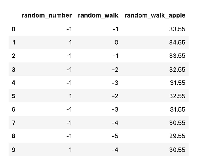
Dataframe with a generated random walk (image by author)
Now, let’s compare randomly generated walk with the actual Apple stock time series:
fig, axes = plt.subplots(nrows=2, ncols=1, figsize=(14, 14))df["adjusted_close"].plot(ax=axes[0])
random_walk["random_walk_apple"].plot(ax=axes[1])
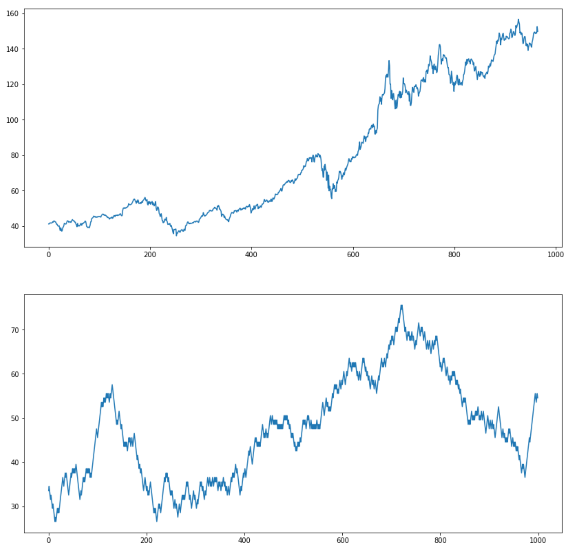
Apple stock time series and random walk (image by author)
I intentionally didn’t include the title on the plots above. Could you tell which is random and which is the actual Apple stock time series?
Is our time series predictable or is it random?
Photo by Universal Eye on Unsplash
To answer this question, we need to compare the properties of the randomly generated sequence with the properties of the Apple stock time series.
One useful tool is the autocorrelation plot, which shows how correlated is each observation with observations from the previous time steps.
Autocorrelation is the correlation of a signal with a delayed copy of itself as a function of delay. Informally, it is the similarity between observations as a function of the time lag between them.
The way random walk is constructed (the current state is calculated as +1 or -1 from the previous state — high dependency on the previous state), we would expect that there would be a high autocorrelation in the first few time steps, which would linearly fall by increasing the lag.
Pandas has an autocorrelation_plot function, which calculates autocorrelation and visualizes it on an autocorrelation plot.
Let’s visualize autocorrelation plots for the random walk and the Apple stock time series.
fig, axes = plt.subplots(nrows=2, ncols=1, figsize=(14, 14))axes[0].set_title("Autocorrelation plot for Apple stock time series")
pd.plotting.autocorrelation_plot(df["adjusted_close"], ax=axes[0])axes[1].set_title("Autocorrelation plot for random walk time series")
pd.plotting.autocorrelation_plot(random_walk["random_walk_apple"], ax=axes[1])
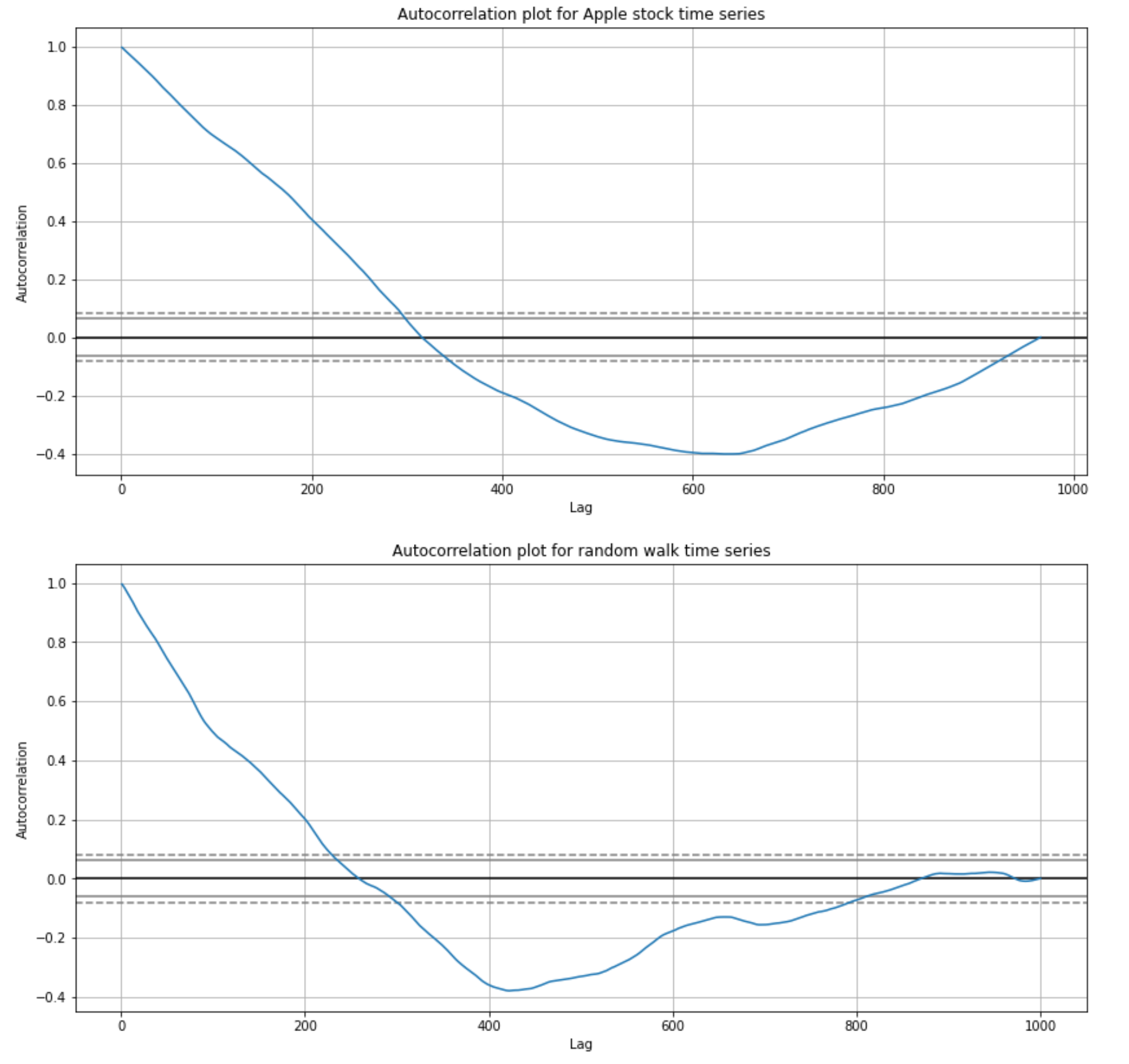
Autocorrelation plots for the random walk and the Apple stock time series (image by author)
The plot shows autocorrelation on the x-axis and lag on the y-axis. The horizontal lines in the plot correspond to 95% and 99% confidence bands. The dashed line is 99%, confidence band. Values above these lines are statistically significant.
As we expected for the random walk sequence, there is a high autocorrelation in the first 100 time steps, which linearly falls with increasing lag.
Surprisingly (or not surprisingly to some), the autocorrelation on the Apple stock time series is similar to the random walk autocorrelation plot.
Put Deep Neural Nets back to sleep…

Photo by Pierre Bamin on Unsplash
Let’s make both time series stationary by removing the value of the previous observation from the current observation — differencing. By applying differencing operation we remove the function of time.
Commands below apply differencing operating to Apple stock and random walk time series:
# applying differencing operation
# [1:] is used to remove the first value which is nullapple_stationary = df["adjusted_close"].diff()[1:]
random_walk_stationary = random_walk["random_walk_apple"].diff()[1:]
Differenced Apple stock time series (image by author)
Now, let’s visualize differenced time series:
fig, axes = plt.subplots(nrows=2, ncols=1, figsize=(14, 14))apple_stationary.plot(ax=axes[0], title="Differenced time series of Apple stock")random_walk_stationary.plot(ax=axes[1], title="Differenced time series of Random walk")
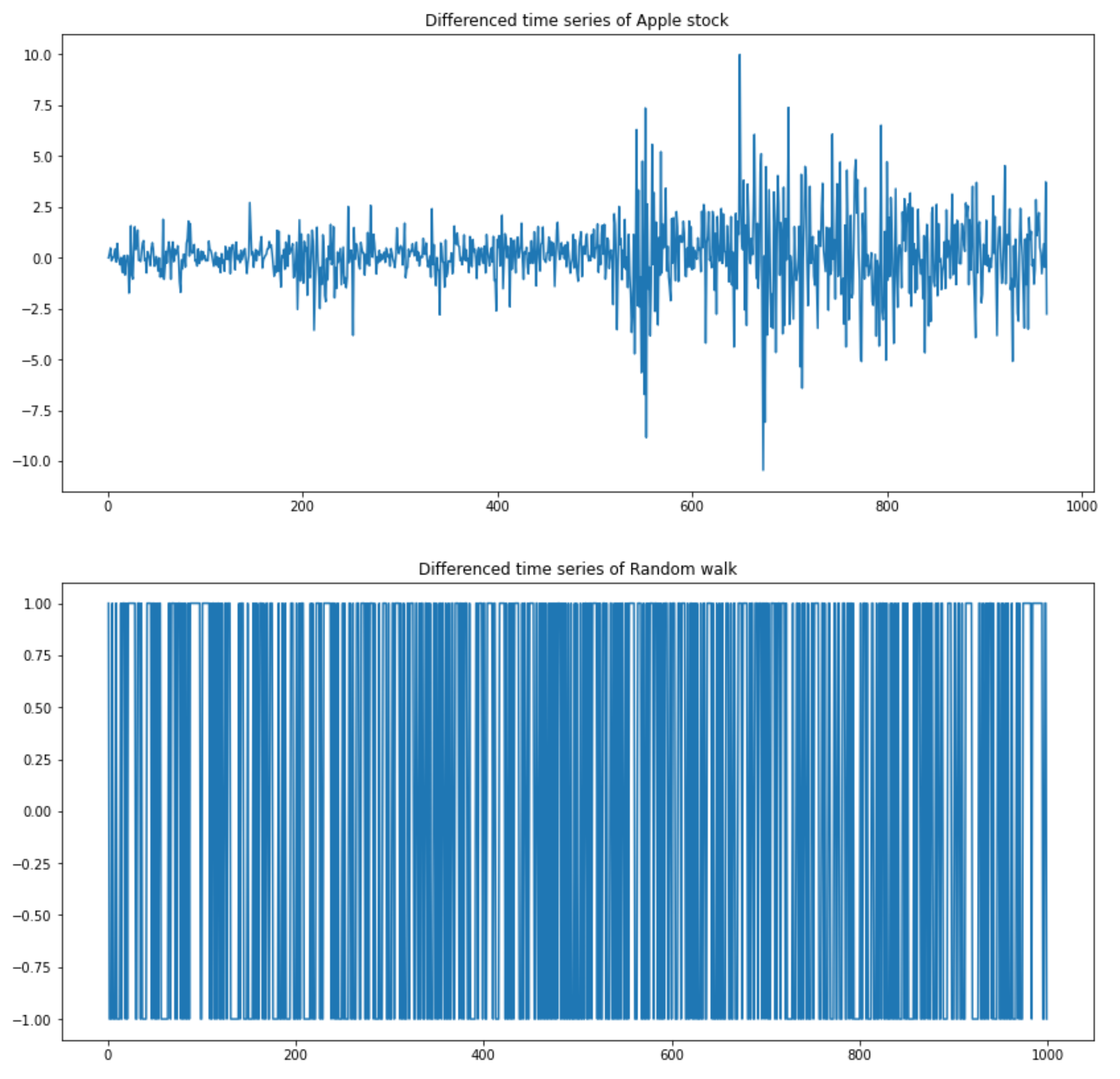
Differenced time series of Apple stock and random walk (image by author)
Differenced random walk time series has only -1 and +1 as expected. Differenced Apple stock time series has more spikes, but are they significant?
We can check this with an autocorrelation plot on a differenced time series:
fig, axes = plt.subplots(nrows=2, ncols=1, figsize=(14, 14))pd.plotting.autocorrelation_plot(apple_stationary, ax=axes[0])
pd.plotting.autocorrelation_plot(random_walk_stationary, ax=axes[1])
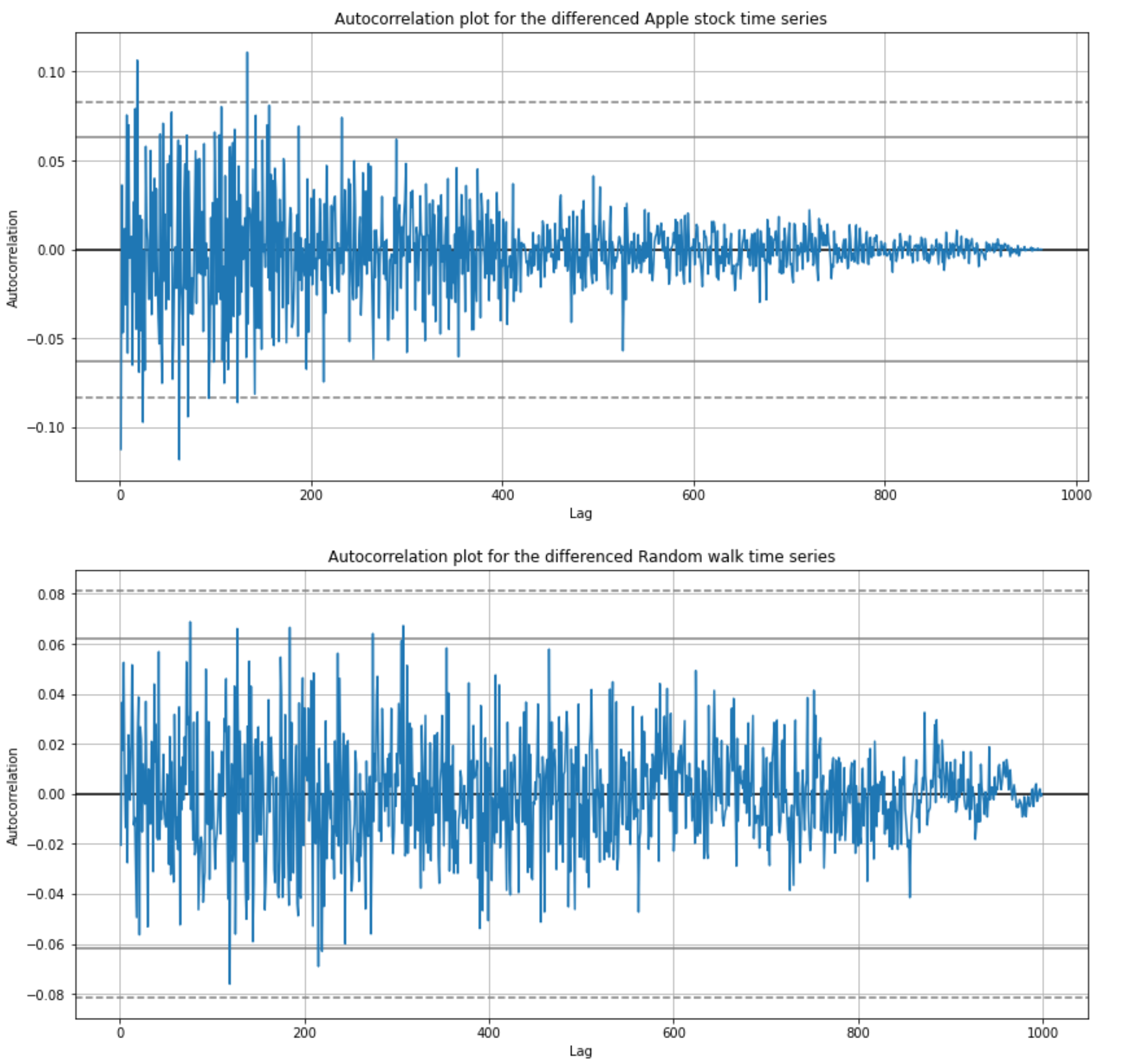
Autocorrelation plots for the differenced random walk and the Apple stock time series (image by author)
Remember, autocorrelation values above horizontal lines are statistically significant.
Differenced Apple stock time series has a few autocorrelation values that are over the 99% confidence band, but also differenced random walk time series has a few values over the 95% confidence band and we know that the signal is random so we can attribute these to statistical mistakes.
Conclusion
Photo by Ferdinand Stöhr on Unsplash
In the article, we applied a few statistical checks on real-world time series data and we determined that the signal from it is random.
What are my two cents on this?
You were probably surprised (as I was) that we didn’t find any statistically significant signal in the Apply stock time series.
How is that possible when we constantly hear stories on how Machine Learning algorithms are used to make automated decisions on the stock market?
Well, while I’m sure Machine Learning algorithms are used to make such decisions — Marcos López de Prado wrote a whole book on this topic — I’m also sure that they use more data. And I don’t mean more price data, but a different kind of data, which influenced the stock price movements.
You can read the Random walk hypothesis on Wikipedia, which states that stock market prices evolve according to a random walk (so price changes are random) and thus cannot be predicted.
What are your thoughts about this? Let me know in the comments below.
Bio: Roman Orac is a Machine Learning engineer with notable successes in improving systems for document classification and item recommendation. Roman has experience with managing teams, mentoring beginners and explaining complex concepts to non-engineers.
Original. Reposted with permission.
Related:
- Top 5 Time Series Methods
- Advice to aspiring Data Scientists – your most common questions answered
- Multivariate Time Series Analysis with an LSTM based RNN