Pandas GroupBy Explained With Examples

# Introduction

 
Pandas is one of the most popular Python libraries for data analysis. It gives you simple tools for cleaning, reshaping, summarizing, and exploring structured data. One of the most useful features in pandas is GroupBy. It helps you answer questions that require grouping rows by one or more categories.

For example, if you are working with sales data, you may want to calculate total revenue by region, average order value by product category, or the number of orders handled by each sales representative. Instead of manually filtering each category one by one, GroupBy lets you perform these calculations in a clean and efficient way.

In this tutorial, we will walk through practical examples of using Pandas GroupBy with a small sales dataset. I am using Deepnote as the coding environment, so some outputs are shown as notebook screenshots directly under the code blocks.

# Creating a Sample Dataset

 
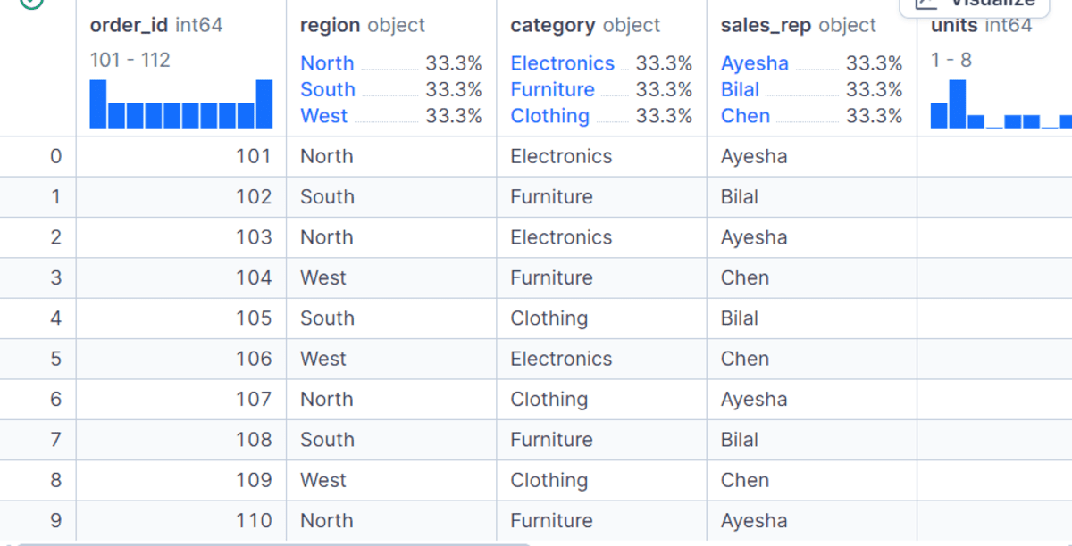
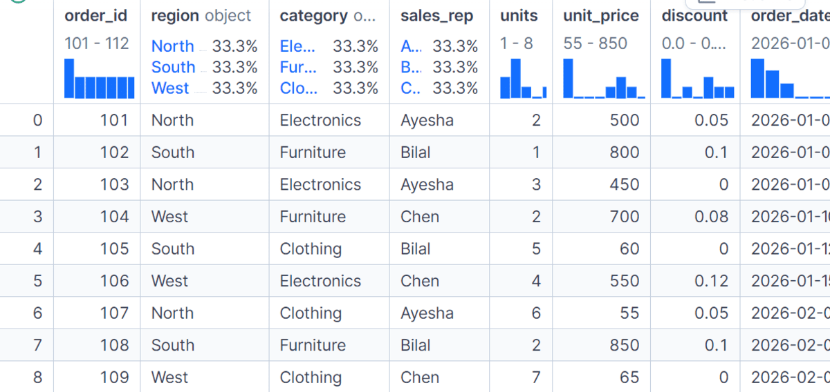
Before using GroupBy, we first create a small retail sales dataset with columns such as order_id, region, category, sales_rep, units, unit_price, discount, and order_date. We then convert the dictionary into a pandas DataFrame and create two new columns: gross_sales and net_sales.

data = {
    "order_id": [101, 102, 103, 104, 105, 106, 107, 108, 109, 110, 111, 112],
    "region": ["North", "South", "North", "West", "South", "West", "North", "South", "West", "North", "South", "West"],
    "category": ["Electronics", "Furniture", "Electronics", "Furniture", "Clothing", "Electronics",
                 "Clothing", "Furniture", "Clothing", "Furniture", "Electronics", "Clothing"],
    "sales_rep": ["Ayesha", "Bilal", "Ayesha", "Chen", "Bilal", "Chen",
                  "Ayesha", "Bilal", "Chen", "Ayesha", "Bilal", "Chen"],
    "units": [2, 1, 3, 2, 5, 4, 6, 2, 7, 1, 2, 8],
    "unit_price": [500, 800, 450, 700, 60, 550, 55, 850, 65, 750, 520, 70],
    "discount": [0.05, 0.10, 0.00, 0.08, 0.00, 0.12, 0.05, 0.10, 0.00, 0.07, 0.03, 0.00],
    "order_date": pd.to_datetime([
        "2026-01-05", "2026-01-06", "2026-01-08", "2026-01-10",
        "2026-01-12", "2026-01-15", "2026-02-02", "2026-02-05",
        "2026-02-08", "2026-02-12", "2026-02-15", "2026-02-20"
    ])
}

df = pd.DataFrame(data)

df["gross_sales"] = df["units"] * df["unit_price"]
df["net_sales"] = df["gross_sales"] * (1 - df["discount"])

df

The gross_sales column is calculated by multiplying units by unit_price, while net_sales adjusts that value after applying the discount. This gives us a clean dataset that we can use for all GroupBy examples.

# Using the Basic GroupBy Syntax

 
The most basic GroupBy operation follows a simple pattern: select a grouping column, select the value column, and apply an aggregation function. In this example, we group the data by region and calculate the total net_sales for each region.

df.groupby("region")["net_sales"].sum()

The result shows that North, South, and West each have their own total sales value. This is the simplest and most common use case for GroupBy when summarizing data.

region
North    3311.0
South    3558.8
West     4239.0
Name: net_sales, dtype: float64

# Using GroupBy With as_index=False

 
By default, pandas uses the grouped column as the index in the output. While this is useful in some cases, it is often easier to work with a normal DataFrame where the grouped column remains a regular column. That is where as_index=False is useful.

df.groupby("region", as_index=False)["net_sales"].sum()

In this example, we again calculate total net sales by region, but the result is returned as a clean DataFrame, which is easier to export, merge, or use in reports.

# Applying Multiple Aggregations on One Column

 
GroupBy is not limited to a single calculation. You can apply multiple aggregation functions to the same column using agg().

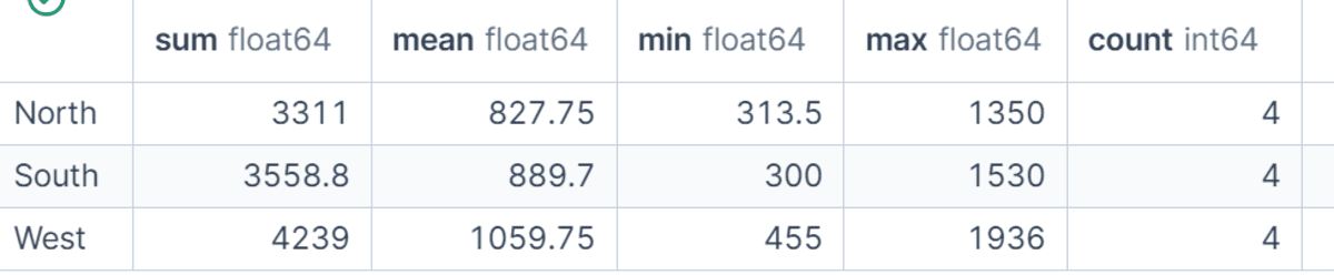
In this example, we calculate the sum, mean, minimum, maximum, and count of net_sales for each region.

This gives us a quick statistical summary of regional sales performance and helps us compare not only total revenue but also average order size and order volume.

df.groupby("region")["net_sales"].agg(["sum", "mean", "min", "max", "count"])

# Using Named Aggregations

 
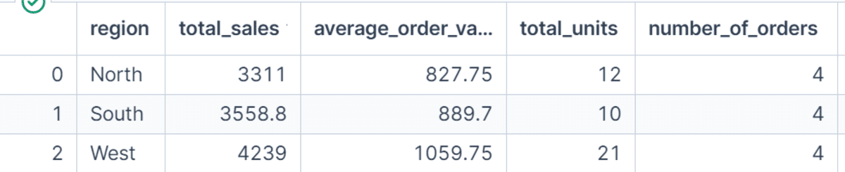
Named aggregations make GroupBy outputs easier to read and use. Instead of returning generic column names like sum or mean, we define our own names such as total_sales, average_order_value, total_units, and number_of_orders.

This is especially helpful when preparing analysis for dashboards, reports, or tutorials because the output column names clearly explain what each metric represents.

region_summary = (
    df.groupby("region", as_index=False)
      .agg(
          total_sales=("net_sales", "sum"),
          average_order_value=("net_sales", "mean"),
          total_units=("units", "sum"),
          number_of_orders=("order_id", "count")
      )
)

region_summary

# Grouping by Multiple Columns

 
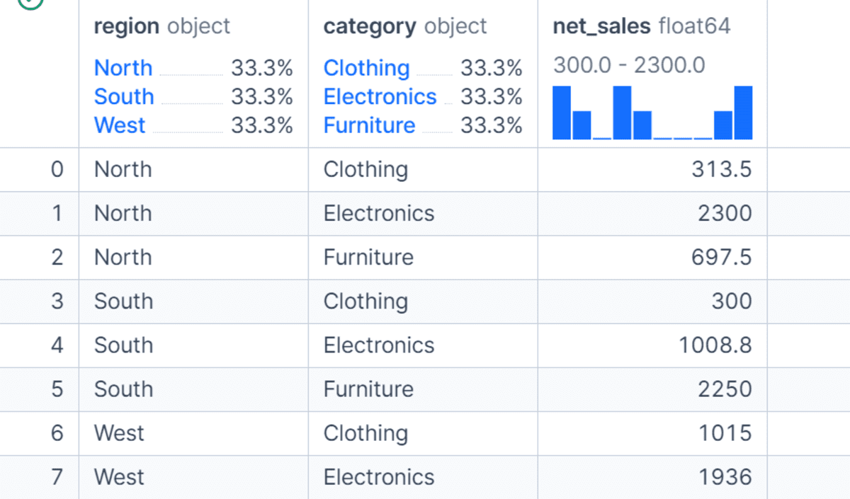
You can also group data by more than one column. In this example, we group by both region and category to calculate total net sales for each product category within each region.

This gives us a more detailed view of the data compared to grouping by region alone. Multi-column grouping is useful when you want to analyze performance across different dimensions, such as region and product, department and employee, or month and customer segment.

df.groupby(["region", "category"], as_index=False)["net_sales"].sum()

# Sorting GroupBy Results

 
After grouping and aggregating data, you often want to sort the results to find the highest or lowest values.

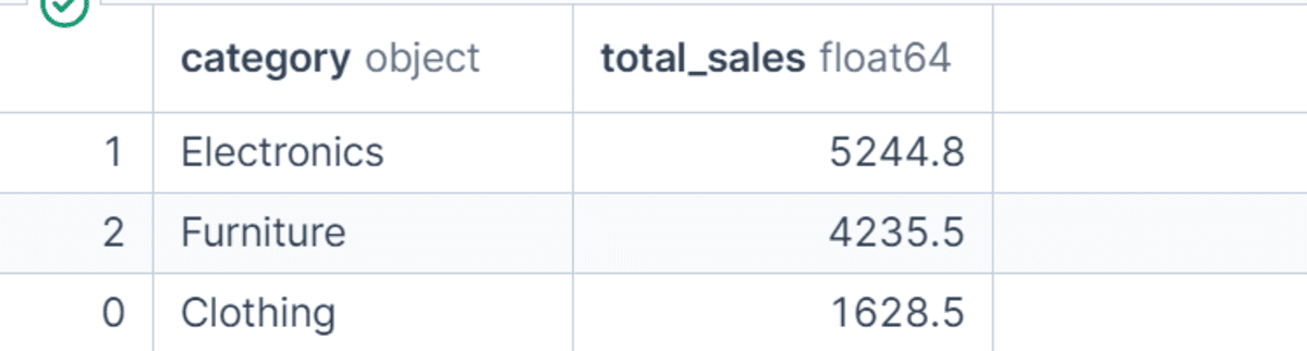
In this example, we calculate total sales by product category and then sort the results in descending order.

This makes it easy to identify which category generated the most revenue. Sorting grouped results is a simple but powerful step when turning raw summaries into useful insights.

category_sales = (
    df.groupby("category", as_index=False)
      .agg(total_sales=("net_sales", "sum"))
      .sort_values("total_sales", ascending=False)
)

category_sales

# Understanding Count vs Size

 
Pandas provides both count() and size(), but they are not exactly the same. The size() method counts the total number of rows in each group, including rows with missing values. The count() method counts only non-missing values in a selected column.

In this example, we intentionally add a missing value to the sales_rep column. The output shows that size() still counts four rows for each region, while count() returns three for North because one sales_rep value is missing.

import numpy as np

df_missing = df.copy()
df_missing.loc[2, "sales_rep"] = np.nan

print("Using size():")
display(df_missing.groupby("region").size())

print("Using count() on sales_rep:")
display(df_missing.groupby("region")["sales_rep"].count())

Output:

Using size():
region
North    4
South    4
West     4
dtype: int64

Using count() on sales_rep:
region
North    3
South    4
West     4
Name: sales_rep, dtype: int64

# Using transform() for Group-Level Features

 
The transform() method is useful when you want to calculate a group-level value and add it back to the original DataFrame.

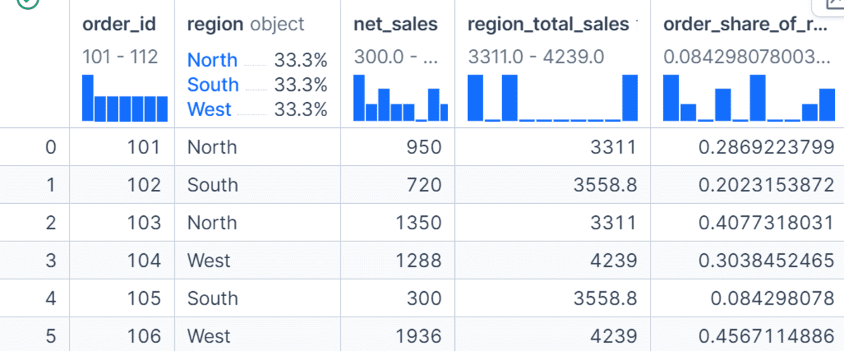
In this example, we calculate total sales for each region and store it in a new column called region_total_sales.

We then calculate each order's share of its region's total sales. Unlike agg(), which reduces the data to one row per group, transform() returns values aligned with the original rows, making it very useful for feature engineering.

df["region_total_sales"] = df.groupby("region")["net_sales"].transform("sum")
df["order_share_of_region"] = df["net_sales"] / df["region_total_sales"]

df[["order_id", "region", "net_sales", "region_total_sales", "order_share_of_region"]]

# Filtering Groups With filter()

 
The filter() method lets you keep or remove entire groups based on a condition. In this example, we keep only the regions where total net sales are greater than 3,000.

Instead of returning one summary row per group, filter() returns the original rows from the groups that meet the condition. This is useful when you want to remove low-performing groups or keep only groups that satisfy a business rule.

high_sales_regions = df.groupby("region").filter(lambda group: group["net_sales"].sum() > 3000)

high_sales_regions

# Applying Custom Logic With apply()

 
The apply() method gives you more flexibility because it allows you to run custom logic on each group.

In this example, we use apply() with nlargest() to find the top order by net sales in each region. This is useful when built-in aggregation functions are not enough for your analysis.

However, apply() can be slower than built-in methods like sum(), mean(), agg(), and transform(), so it is best to use it only when you need custom group-wise operations.

top_order_by_region = (
    df.groupby("region", group_keys=False)
      .apply(lambda group: group.nlargest(1, "net_sales"))
)

top_order_by_region

# Grouping by Dates

 
GroupBy is also very useful for time-based analysis.

In this example, we extract the month from the order_date column and group the data by month.

We then calculate total sales and total orders for each month. This approach is helpful when analyzing trends over time, such as monthly sales, weekly user activity, or yearly revenue growth.

df["month"] = df["order_date"].dt.to_period("M").astype(str)

monthly_sales = (
    df.groupby("month", as_index=False)
      .agg(total_sales=("net_sales", "sum"), total_orders=("order_id", "count"))
)

monthly_sales

# Grouping by Dates With pd.Grouper

 
pd.Grouper provides a cleaner way to group time series data without manually creating a separate month column.

In this example, we group the DataFrame by order_date using a monthly frequency and calculate total sales and total orders.

This is especially useful when working with real-world datasets that contain timestamps and you want to summarize data by day, week, month, quarter, or year.

monthly_sales_grouper = (
    df.groupby(pd.Grouper(key="order_date", freq="M"))
      .agg(total_sales=("net_sales", "sum"), total_orders=("order_id", "count"))
      .reset_index()
)

monthly_sales_grouper

# Creating a Pivot-Style Summary With GroupBy

 
You can combine groupby() with unstack() to create a pivot-style summary table.

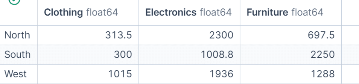
In this example, we group the data by region and category, calculate total net sales, and then reshape the result so that categories become columns. This makes the output easier to compare across regions and categories. It is a great technique when you want a compact table for reporting or quick analysis.

region_category_table = (
    df.groupby(["region", "category"])["net_sales"]
      .sum()
      .unstack(fill_value=0)
)

region_category_table

# Conclusion

 
Pandas GroupBy is one of the most powerful tools for data analysis in Python. It helps you summarize data, compare groups, create new features, filter results, and apply custom calculations without writing unnecessary manual logic.

While working on this tutorial, I realized how much depth there is in GroupBy. Even after working with data for years, I learned new and better ways to solve common problems. Features like pd.Grouper, custom aggregation functions, and transform() stood out because they make many tasks faster, cleaner, and easier to maintain.

This is also why understanding the native tools matters. It is tempting to rely on vibe coding or quick custom solutions, but those can often produce slower, more complicated code. When you know what pandas already provides, you can write solutions that are more efficient, reusable, and practical for real-world data analysis.

In this tutorial, we covered the most useful GroupBy operations, including basic aggregation, named aggregation, multi-column grouping, sorting, count() vs size(), transform(), filter(), apply(), date grouping, and pivot-style summaries. Once you understand these patterns, you can use GroupBy to answer many real-world data analysis questions quickly and confidently.
 
 

Abid Ali Awan (@1abidaliawan) is a certified data scientist professional who loves building machine learning models. Currently, he is focusing on content creation and writing technical blogs on machine learning and data science technologies. Abid holds a Master's degree in technology management and a bachelor's degree in telecommunication engineering. His vision is to build an AI product using a graph neural network for students struggling with mental illness.