Postgres vs MySQL vs SQLite: Comparing SQL Performance Across Engines

Image by Author

# Introduction

 
When designing an application, choosing the right SQL database engine can have a major impact on performance.

Three common options are PostgreSQL, MySQL, and SQLite. Each of these engines has unique strengths and optimization strategies that make it suitable for different scenarios.

PostgreSQL typically excels in dealing with complex analytical queries, and MySQL can also deliver robust general-purpose performance. On the other hand, SQLite offers a lightweight solution for embedded applications.

In this article, we'll benchmark these three engines using four analytical interview questions: two at medium difficulty and two at hard difficulty.

In each of them, the goal is to examine how each engine handles joins, window functions, date arithmetic, and complex aggregations. This will highlight platform-specific optimization strategies and offer useful insights into each engine's performance and specifications.

# Understanding The Three SQL Engines

 
Before diving into the benchmarks, let’s try to understand the differences between these three database systems.

PostgreSQL is a feature-rich, open-source relational database known for advanced SQL compliance and sophisticated query optimization. It can handle complex analytical queries effectively, has strong support for window functions, CTEs, and multiple indexing strategies.

MySQL is the most widely used open-source database, favored for its speed and accuracy in web applications. Despite its historical emphasis on transactional workloads, modern versions of this engine include comprehensive analytical capabilities with window functions and improved query optimization.

SQLite is a lightweight engine embedded directly into applications. Unlike the two previous engines, which run as separate server processes, SQLite runs as a library, making it perfect for mobile applications, desktop programs, and development settings.

However, as you may expect, this simplicity comes with some limitations, for example, in concurrent write operations and certain SQL features.

This article’s benchmark uses four interview questions that test different SQL capabilities.
For each problem, we'll analyze the query solutions across all three engines, highlighting their syntax variations, performance considerations, and optimization opportunities.

We will test their performance regarding execution time. Postgres and MySQL were benchmarked on StrataScratch's platform (server-based), while SQLite was benchmarked locally in memory.

# Solving Medium-Level Questions

// Answering Interview Question #1: Risky Projects

This interview question asks you to identify projects that exceed their budget based on prorated employee salaries.

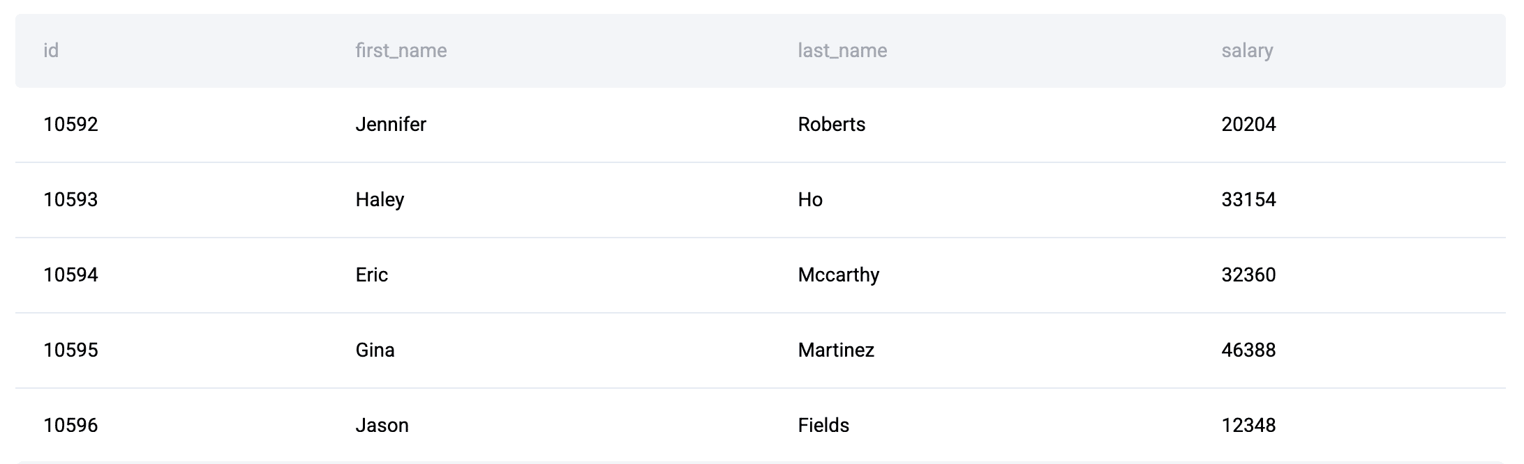
Data Tables: You're given three tables: linkedin_projects (with budgets and dates), linkedin_emp_projects, and linkedin_employees.

 

 

 

 
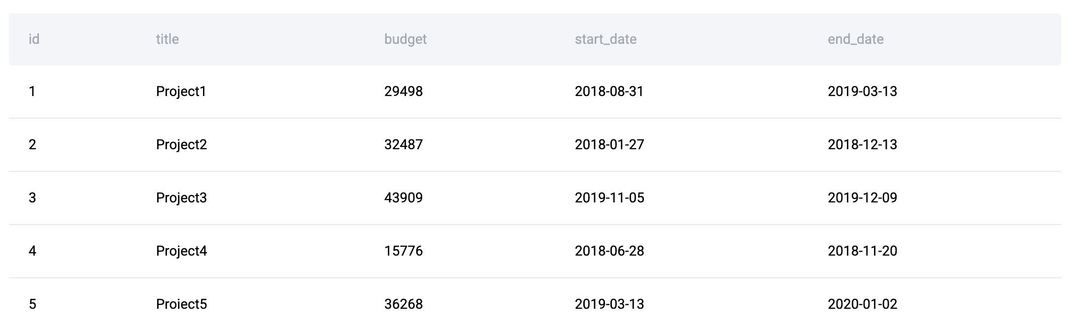
The goal is to compute the portion of each employee's annual salary allocated to each project and to determine which projects are over budget.

In PostgreSQL, the solution is as follows:

SELECT a.title,
       a.budget,
       CEILING((a.end_date - a.start_date) * SUM(c.salary) / 365) AS prorated_employee_expense
FROM linkedin_projects a
INNER JOIN linkedin_emp_projects b ON a.id = b.project_id
INNER JOIN linkedin_employees c ON b.emp_id = c.id
GROUP BY a.title,
         a.budget,
         a.end_date,
         a.start_date
HAVING CEILING((a.end_date - a.start_date) * SUM(c.salary) / 365) > a.budget
ORDER BY a.title ASC;

PostgreSQL handles date arithmetic elegantly with direct subtraction (\( \text{end\_date} - \text{start\_date} \)), which returns the number of days between dates.

The computation is simple and easy to read because of the engine’s native date handling.

In MySQL, the solution is:

SELECT a.title,
       a.budget,
       CEILING(DATEDIFF(a.end_date, a.start_date) * SUM(c.salary) / 365) AS prorated_employee_expense
FROM linkedin_projects a
INNER JOIN linkedin_emp_projects b ON a.id = b.project_id
INNER JOIN linkedin_employees c ON b.emp_id = c.id
GROUP BY a.title,
         a.budget,
         a.end_date,
         a.start_date
HAVING CEILING(DATEDIFF(a.end_date, a.start_date) * SUM(c.salary) / 365) > a.budget
ORDER BY a.title ASC;

In MySQL, the DATEDIFF() function is required for date arithmetic, which explicitly computes how many days are between two dates.

While this adds a function call, MySQL's query optimizer handles this efficiently.

Finally, let’s take a look at the SQLite solution:

SELECT a.title,
    a.budget,
    CAST(
        (julianday(a.end_date) - julianday(a.start_date)) * (SUM(c.salary) / 365) + 0.99
    AS INTEGER) AS prorated_employee_expense
FROM linkedin_projects a
INNER JOIN linkedin_emp_projects b ON a.id = b.project_id
INNER JOIN linkedin_employees c ON b.emp_id = c.id
GROUP BY a.title, a.budget, a.end_date, a.start_date
HAVING CAST(
        (julianday(a.end_date) - julianday(a.start_date)) * (SUM(c.salary) / 365) + 0.99
    AS INTEGER) > a.budget
ORDER BY a.title ASC;

SQLite uses the julianday() function to convert dates to numeric values for arithmetic operations.

Because SQLite does not have a CEILING() function, we can mimic it by adding 0.99 and converting to an integer, which rounds up accurately.

// Optimizing Queries

For each of the three engines, indexes may be used on join columns (project_id, emp_id, id) to improve performance dramatically. PostgreSQL's advantages arise from the use of composite indexes on (title, budget, end_date, start_date) for the GROUP BY clause.

Proper primary key usage is essential, as MySQL's InnoDB engine automatically clusters data by the primary key.

// Answering Interview Question #2: Finding User Purchases

The goal of this interview question is to output the IDs of repeat customers who made a second purchase within 1 to 7 days after their first purchase (excluding same-day repurchases).

Data Tables: The only table is amazon_transactions. It contains transaction records with id, user_id, item, created_at, and revenue.

 

 
PostgreSQL Solution:

WITH daily AS (
    SELECT DISTINCT user_id, created_at::date AS purchase_date
    FROM amazon_transactions
),
ranked AS (
    SELECT user_id, purchase_date,
        ROW_NUMBER() OVER (PARTITION BY user_id ORDER BY purchase_date) AS rn
    FROM daily
),
first_two AS (
    SELECT user_id,
        MAX(CASE WHEN rn = 1 THEN purchase_date END) AS first_date,
        MAX(CASE WHEN rn = 2 THEN purchase_date END) AS second_date
    FROM ranked
    WHERE rn <= 2
    GROUP BY user_id
)
SELECT user_id
FROM first_two
WHERE second_date IS NOT NULL
    AND (second_date - first_date) BETWEEN 1 AND 7
ORDER BY user_id;

In PostgreSQL, the solution is to use CTEs (Common Table Expressions) to break the problem into logical and readable steps.

The date cast function turns timestamps into dates, while the window functions with ROW_NUMBER() rank purchases chronologically. The inherent date subtraction feature of PostgreSQL keeps the final filter tidy and effective.

MySQL Solution:

WITH daily AS (
    SELECT DISTINCT user_id, DATE(created_at) AS purchase_date
    FROM amazon_transactions
),
ranked AS (
    SELECT user_id, purchase_date,
        ROW_NUMBER() OVER (PARTITION BY user_id ORDER BY purchase_date) AS rn
    FROM daily
),
first_two AS (
    SELECT user_id,
        MAX(CASE WHEN rn = 1 THEN purchase_date END) AS first_date,
        MAX(CASE WHEN rn = 2 THEN purchase_date END) AS second_date
    FROM ranked
    WHERE rn <= 2
    GROUP BY user_id
)
SELECT user_id
FROM first_two
WHERE second_date IS NOT NULL
    AND DATEDIFF(second_date, first_date) BETWEEN 1 AND 7
ORDER BY user_id;

MySQL’s solution is similar to the previous PostgreSQL structure, using CTEs and window functions.

The main difference here is the use of the DATE() and DATEDIFF() functions for date extraction and comparison. MySQL 8.0+ supports CTEs efficiently, whereas earlier versions require subqueries.

SQLite Solution:

WITH daily AS (
    SELECT DISTINCT user_id, DATE(created_at) AS purchase_date
    FROM amazon_transactions
),
ranked AS (
    SELECT user_id, purchase_date,
        ROW_NUMBER() OVER (PARTITION BY user_id ORDER BY purchase_date) AS rn
    FROM daily
),
first_two AS (
    SELECT user_id,
        MAX(CASE WHEN rn = 1 THEN purchase_date END) AS first_date,
        MAX(CASE WHEN rn = 2 THEN purchase_date END) AS second_date
    FROM ranked
    WHERE rn <= 2
    GROUP BY user_id
)
SELECT user_id
FROM first_two
WHERE second_date IS NOT NULL
    AND (julianday(second_date) - julianday(first_date)) BETWEEN 1 AND 7
ORDER BY user_id;

SQLite (version 3.25+) also supports CTEs and window functions, making the structure identical to the two previous ones. In this case, the only difference is the date arithmetic, which uses julianday() instead of native subtraction or DATEDIFF().

// Optimizing Queries

Indexes can also be used in this case for efficient partitioning in window functions, specifically for the user_id. PostgreSQL can benefit from partial indexes on active users.
If working with large datasets, one may also consider materializing the daily CTE in PostgreSQL. For optimal CTE performance in MySQL, ensure you're using version 8.0+.

# Solving Hard-Level Questions

// Answering Interview Question #3: Revenue Over Time

This interview question asks you to compute a 3-month rolling average of total revenue from purchases.

The goal is to output year-month values with their corresponding rolling averages, sorted chronologically. Returns (negative purchase amounts) should be excluded.

Data Tables:
amazon_purchases: Contains purchase records with user_id, created_at, and purchase_amt

 

 
First, let’s check the PostgreSQL solution:

SELECT t.month,
    AVG(t.monthly_revenue) OVER(
        ORDER BY t.month 
        ROWS BETWEEN 2 PRECEDING AND CURRENT ROW
    ) AS avg_revenue
FROM (
    SELECT to_char(created_at::date, 'YYYY-MM') AS month,
        sum(purchase_amt) AS monthly_revenue
    FROM amazon_purchases
    WHERE purchase_amt > 0
    GROUP BY to_char(created_at::date, 'YYYY-MM')
    ORDER BY to_char(created_at::date, 'YYYY-MM')
) t
ORDER BY t.month ASC;

PostgreSQL outperforms with window functions, as the frame specification ROWS BETWEEN 2 PRECEDING AND CURRENT ROW defines the rolling window precisely.
The to_char() function formats dates into year-month strings for grouping.

Next, the MySQL Solution:

SELECT t.`month`,
    AVG(t.monthly_revenue) OVER(
        ORDER BY t.`month` 
        ROWS BETWEEN 2 PRECEDING AND CURRENT ROW
    ) AS avg_revenue
FROM (
    SELECT DATE_FORMAT(created_at, '%Y-%m') AS month,
        sum(purchase_amt) AS monthly_revenue
    FROM amazon_purchases
    WHERE purchase_amt > 0
    GROUP BY DATE_FORMAT(created_at, '%Y-%m')
    ORDER BY DATE_FORMAT(created_at, '%Y-%m')
) t
ORDER BY t.`month` ASC;

MySQL's implementation handles the window function identically, although it uses the DATE_FORMAT() function instead of to_char().

Note this engine has a specific syntax requirement to avoid keyword conflicts, hence the backticks around month.

Finally, the SQLite solution is:

SELECT t.month,
    AVG(t.monthly_revenue) OVER(
        ORDER BY t.month 
        ROWS BETWEEN 2 PRECEDING AND CURRENT ROW
    ) AS avg_revenue
FROM (
    SELECT strftime('%Y-%m', created_at) AS month,
        SUM(purchase_amt) AS monthly_revenue
    FROM amazon_purchases
    WHERE purchase_amt > 0
    GROUP BY strftime('%Y-%m', created_at)
    ORDER BY strftime('%Y-%m', created_at)
) t
ORDER BY t.month ASC;

Date formatting in SQLite requires the usage of strftime(), and this engine supports the same window function syntax as PostgreSQL and MySQL (in version 3.25+). Performance is comparable for small to medium-sized datasets.

// Optimizing Queries

Window functions can be computationally expensive to use.

For PostgreSQL, consider creating an index on created_at and, if this query runs frequently, a materialized view for monthly aggregation.

MySQL benefits from covering indexes that include both created_at and purchase_amt.

For SQLite, you need to be using version 3.25 or later to have window function support.

// Answering Interview Question #4: Common Friends’ Friend

Moving on to the next interview question, this one asks you to find the count of each user's friends who are also friends with the user's other friends (essentially, mutual connections within a network). The goal is to output user IDs with the count of these common friend-of-friend relationships.

Data Tables:
google_friends_network: Contains friendship relationships with user_id and friend_id.

 

 
The PostgreSQL solution is:

WITH bidirectional_relationship AS (
    SELECT user_id, friend_id
    FROM google_friends_network
    UNION
    SELECT friend_id AS user_id, user_id AS friend_id
    FROM google_friends_network
)
SELECT user_id, COUNT(DISTINCT friend_id) AS n_friends
FROM (
    SELECT DISTINCT a.user_id, c.user_id AS friend_id
    FROM bidirectional_relationship a
    INNER JOIN bidirectional_relationship b ON a.friend_id = b.user_id
    INNER JOIN bidirectional_relationship c ON b.friend_id = c.user_id
        AND c.friend_id = a.user_id
) base
GROUP BY user_id;

In PostgreSQL, this complex multi-join query is handled efficiently by its sophisticated query planner.

The initial CTE creates a two-way view of connections within the network, followed by three self-joins that identify triangular relationships in which \( A \) is friends with \( B \), \( B \) is friends with \( C \), and \( C \) is also friends with \( A \).

MySQL Solution:

SELECT user_id, COUNT(DISTINCT friend_id) AS n_friends
FROM (
    SELECT DISTINCT a.user_id, c.user_id AS friend_id
    FROM (
        SELECT user_id, friend_id
        FROM google_friends_network
        UNION
        SELECT friend_id AS user_id, user_id AS friend_id
        FROM google_friends_network
    ) AS a
    INNER JOIN (
        SELECT user_id, friend_id
        FROM google_friends_network
        UNION
        SELECT friend_id AS user_id, user_id AS friend_id
        FROM google_friends_network
    ) AS b ON a.friend_id = b.user_id
    INNER JOIN (
        SELECT user_id, friend_id
        FROM google_friends_network
        UNION
        SELECT friend_id AS user_id, user_id AS friend_id
        FROM google_friends_network
    ) AS c ON b.friend_id = c.user_id
        AND c.friend_id = a.user_id
) base
GROUP BY user_id;

MySQL's solution repeats the UNION subquery three times instead of using a single CTE.

Although less elegant, this is required for MySQL versions prior to 8.0. Modern MySQL versions can use the PostgreSQL approach with CTEs for better readability and potential performance improvements.

SQLite Solution:

WITH bidirectional_relationship AS (
    SELECT user_id, friend_id
    FROM google_friends_network
    UNION
    SELECT friend_id AS user_id, user_id AS friend_id
    FROM google_friends_network
)
SELECT user_id, COUNT(DISTINCT friend_id) AS n_friends
FROM (
    SELECT DISTINCT a.user_id, c.user_id AS friend_id
    FROM bidirectional_relationship a
    INNER JOIN bidirectional_relationship b ON a.friend_id = b.user_id
    INNER JOIN bidirectional_relationship c ON b.friend_id = c.user_id
        AND c.friend_id = a.user_id
) base
GROUP BY user_id;

SQLite supports CTEs and handles this query identically to PostgreSQL.

However, performance may degrade when handling large networks due to SQLite's simpler query optimizer and the absence of advanced indexing strategies.

// Optimizing Queries

For all engines, composite indexes on (user_id, friend_id) can be created to improve performance. In PostgreSQL, we can use hash joins for large datasets when work_mem is configured appropriately.

For MySQL, make sure the InnoDB buffer pool is sized adequately. SQLite may struggle with very large networks. For this, consider denormalizing or pre-computing relationships for production use.

# Comparing Performance

 

 
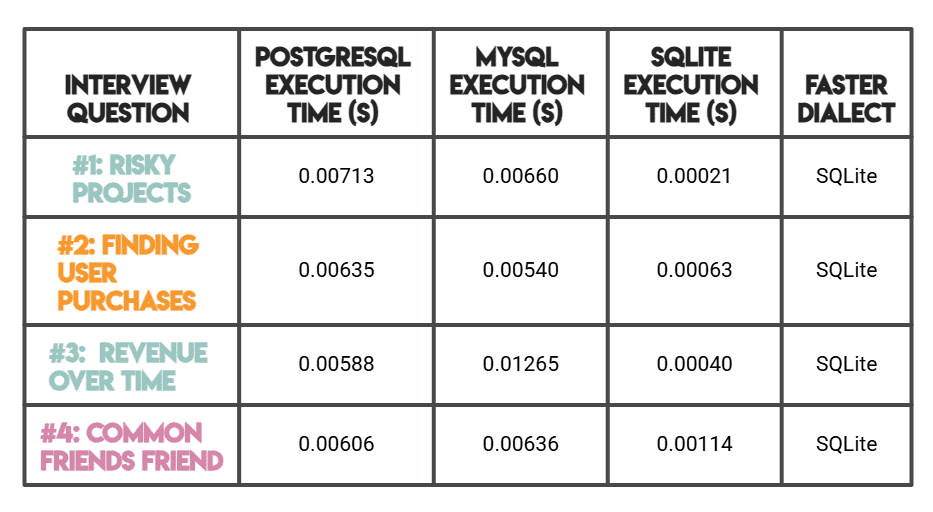
Note: As mentioned before, PostgreSQL and MySQL were benchmarked on StrataScratch's platform (server-based), while SQLite was benchmarked locally in memory.

SQLite's significantly faster times make sense due to its serverless, zero-overhead architecture (rather than superior query optimization).

For a server-to-server comparison, MySQL outperforms PostgreSQL on simpler queries (#1, #2), whereas PostgreSQL is faster on complex analytical workloads (#3, #4).

# Analyzing Key Performance Differences

 
Across these benchmarks, several patterns emerged:

SQLite was the fastest engine across all four questions, often by a significant margin. This is largely due to its serverless, in-memory architecture, with no network overhead or client-server communication; query execution is nearly instantaneous for small datasets.

However, this speed advantage is most pronounced with smaller data volumes.

PostgreSQL demonstrates superior performance compared to MySQL on complex analytical queries, particularly those involving window functions and multiple CTEs (Questions #3 and #4). Its sophisticated query planner and extensive indexing options make it the go-to choice for data warehousing and analytics workloads where query complexity matters more than raw simplicity.

MySQL beats PostgreSQL on the simpler, medium-difficulty queries (#1 and #2), offering competitive performance with straightforward syntax requirements like DATEDIFF(). Its strength lies in high-concurrency transactional workloads, though modern versions also handle analytical queries well.

In short, SQLite shines for lightweight, embedded use cases with small to medium datasets, PostgreSQL is your best bet for complex analytics at scale, and MySQL strikes a solid balance between performance and general-purpose dependability.

# Concluding Remarks

 
From this article, you will understand some of the nuances between PostgreSQL, MySQL, and SQLite, which can enable you to choose the right tool for your specific needs.

 

 
Again, we saw that MySQL delivers a balance between robust performance and general-purpose reliability, whereas PostgreSQL excels in analytical complexity with sophisticated SQL features. At the same time, SQLite offers lightweight simplicity for embedded settings.

By understanding how each engine performs particular SQL operations, you can get better performance than you would by simply choosing the “best” one. Utilize engine-specific features such as MySQL's covering indexes or PostgreSQL's partial indexes, index your join and filter columns, and always use EXPLAIN or EXPLAIN ANALYZE clauses to comprehend query execution plans.

With these benchmarks, you can now hopefully make informed decisions about database selection and optimization strategies that directly impact your implementation’s performance.
 
 

Nate Rosidi is a data scientist and in product strategy. He's also an adjunct professor teaching analytics, and is the founder of StrataScratch, a platform helping data scientists prepare for their interviews with real interview questions from top companies. Nate writes on the latest trends in the career market, gives interview advice, shares data science projects, and covers everything SQL.