Using SQL to Understand Data Science Career Trends
Reveal the Secrets of the Data Science Job Market with SQL.

Image by Author
In a world where data is the new oil, understanding the nuances of a career in data science is more important than ever. Whether you are a data enthusiast looking or a veteran exploring opportunities, using SQL can offer insights into the data science job market.
I hope you are eager to know which data science job titles are the most attractive, or which ones offer the beefiest paychecks. Or perhaps, you're wondering how experience levels tie into data science average salaries?
In this article, we have got all those questions (and more) covered as we go deep into the data science job market. Let’s start!
Dataset Salary Trend
The dataset that we will use in this article is designed to shed light on salary patterns in the Data Science field from 2021 to 2023. By spotlighting elements such as work history, job positions, and corporate locations, it offers crucial insights into wage dispersion in the sector.
This article will find an answer to the following questions:
- What Does the Average Salary Look Like Across Different Experience Levels?
- What are the Most Common Job Titles in Data Science?
- How Does Salary Distribution Vary with Company Size?
- Where are Data Science Jobs Primarily Located Geographically?
- Which Job Titles Offer the Top Salaries in Data Science?
You can download this data from the Kaggle.
1. What Does the Average Salary Look Like Across Different Experience Levels?
In this SQL query, we are finding the average salary for different experience levels. The GROUP BY clause groups the data by experience level and the AVG function calculates the average salary for each group.
This helps to understand how experience in the field influences the earning potential, which is essential for you while planning your career paths in data science. Let’s see the code.
SELECT experience_level, AVG(salary_in_usd) AS avg_salary
FROM salary_data
GROUP BY experience_level;
Now let’s visualize this output by using Python.
Here is the code.
# Import required libraries for plotting
import matplotlib.pyplot as plt
import seaborn as sns
# Set up the style for the graphs
sns.set(style="whitegrid")

# Initialize the list for storing graphs
graphs = []

plt.figure(figsize=(10, 6))
sns.barplot(x='experience_level', y='salary_in_usd', data=df, estimator=lambda x: sum(x) / len(x))
plt.title('Average Salary by Experience Level')
plt.xlabel('Experience Level')
plt.ylabel('Average Salary (USD)')
plt.xticks(rotation=45)
graphs.append(plt.gcf())
plt.show()
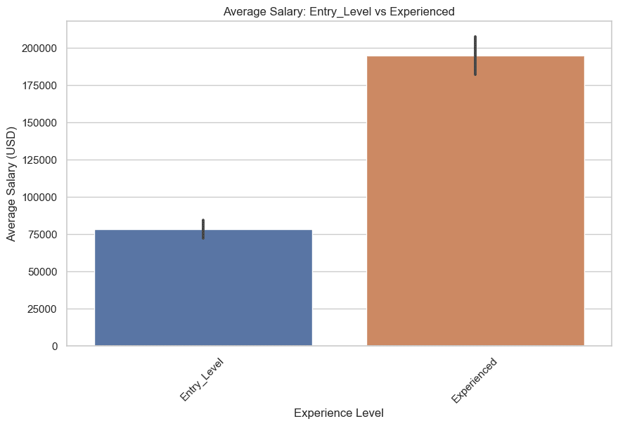
Now let’s compare, entry-level & experienced and mid-level & senior salaries.
Let’s start with entry-level & experienced. Here is the code.
# Filter the data for Entry_Level and Experienced levels
entry_experienced = df[df['experience_level'].isin(['Entry_Level', 'Experienced'])]

# Filter the data for Mid-Level and Senior levels
mid_senior = df[df['experience_level'].isin(['Mid-Level', 'Senior'])]

# Plotting the Entry_Level vs Experienced graph
plt.figure(figsize=(10, 6))
sns.barplot(x='experience_level', y='salary_in_usd', data=entry_experienced, estimator=lambda x: sum(x) / len(x) if len(x) != 0 else 0)
plt.title('Average Salary: Entry_Level vs Experienced')
plt.xlabel('Experience Level')
plt.ylabel('Average Salary (USD)')
plt.xticks(rotation=45)
graphs.append(plt.gcf())
plt.show()
Here is the graph.
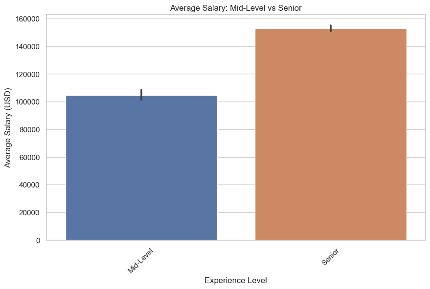
Now let’s draw, mid-level & senior. Here is the code.
# Plotting the Mid-Level vs Senior graph
plt.figure(figsize=(10, 6))
sns.barplot(x='experience_level', y='salary_in_usd', data=mid_senior, estimator=lambda x: sum(x) / len(x) if len(x) != 0 else 0)
plt.title('Average Salary: Mid-Level vs Senior')
plt.xlabel('Experience Level')
plt.ylabel('Average Salary (USD)')
plt.xticks(rotation=45)
graphs.append(plt.gcf())
plt.show()
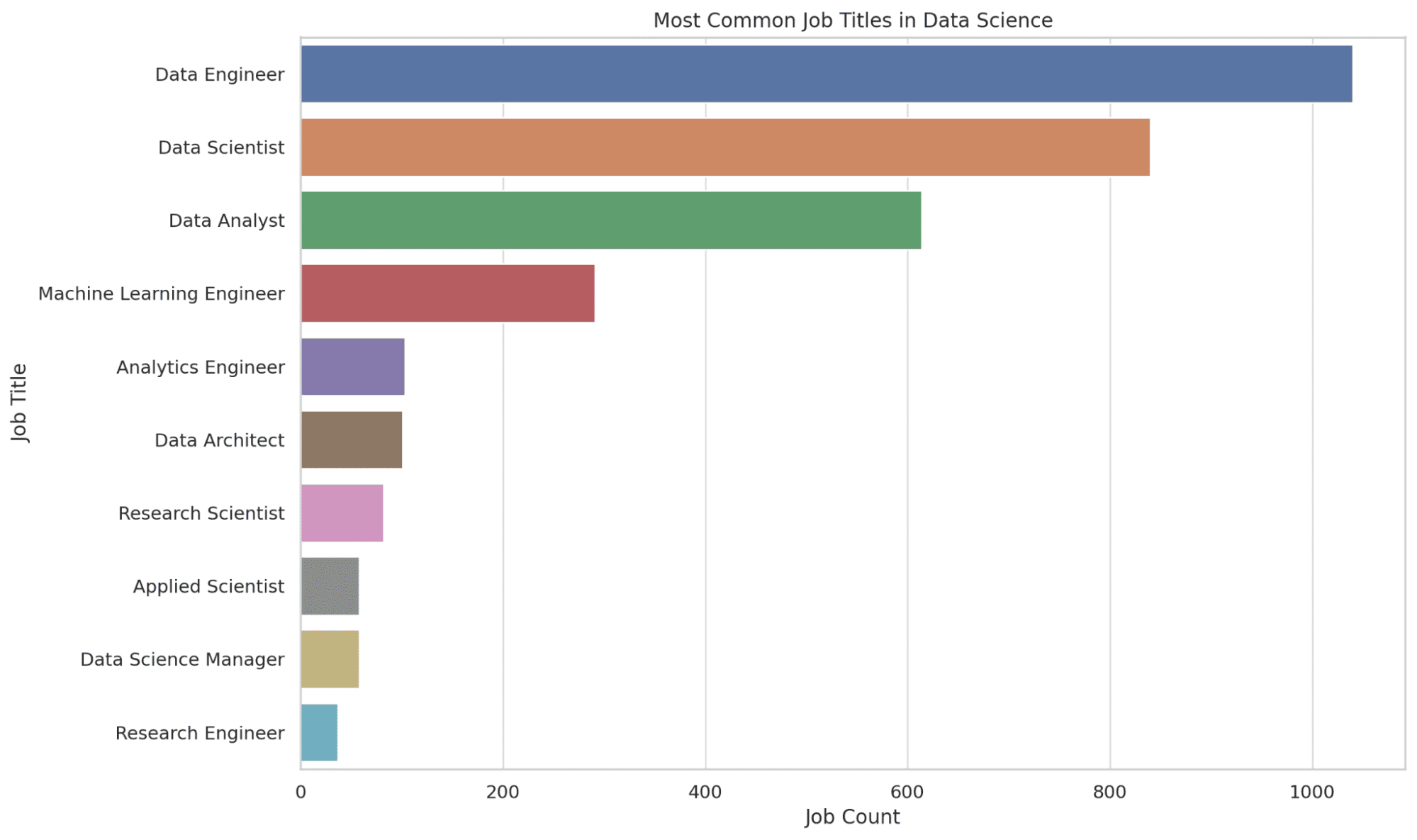
2. What are the Most Common Job Titles in Data Science?
Here, we extract the top 10 most common job titles in data science. The COUNT function counts the number of occurrences of each job title, and the results are ordered in descending order to get the most common titles at the top.
This information gives you a sense of the job market demand, guiding you in identifying potential roles you can target. Let’s see the code.
SELECT job_title, COUNT(*) AS job_count
FROM salary_data
GROUP BY job_title
ORDER BY job_count DESC
LIMIT 10;
Okay, it is time to visualize this query by using Python.
Here is the code.
plt.figure(figsize=(12, 8))
sns.countplot(y='job_title', data=df, order=df['job_title'].value_counts().index[:10])
plt.title('Most Common Job Titles in Data Science')
plt.xlabel('Job Count')
plt.ylabel('Job Title')
graphs.append(plt.gcf())
plt.show()
Let’s see the graph.
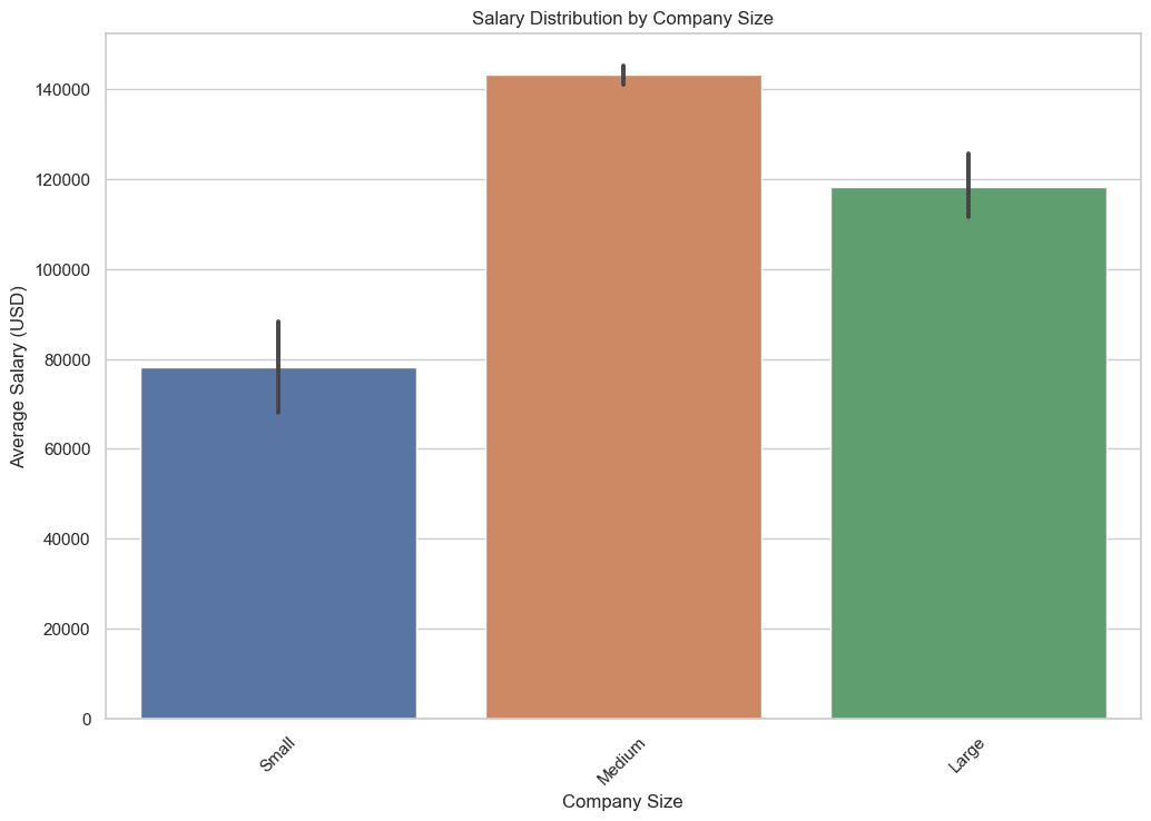
3. How Does Salary Distribution Vary with Company Size?
In this query, we extract the average, minimum, and maximum salaries for each company size grouping. Using aggregate functions such as AVG, MIN, and MAX helps to provide a comprehensive view of the salary landscape in relation to the size of a company.
This data is essential as it helps you understand the potential earnings you can expect depending on the size of the company you are looking to join, let’s see the code.
SELECT company_size, AVG(salary_in_usd) AS avg_salary, MIN(salary_in_usd) AS min_salary, MAX(salary_in_usd) AS max_salary
FROM salary_data
GROUP BY company_size;
Now let’s visualize this query, by using Python.
Here is the code.
plt.figure(figsize=(12, 8))
sns.barplot(x='company_size', y='salary_in_usd', data=df, estimator=lambda x: sum(x) / len(x) if len(x) != 0 else 0, order=['Small', 'Medium', 'Large'])
plt.title('Salary Distribution by Company Size')
plt.xlabel('Company Size')
plt.ylabel('Average Salary (USD)')
plt.xticks(rotation=45)
graphs.append(plt.gcf())
plt.show()
Here is the output.
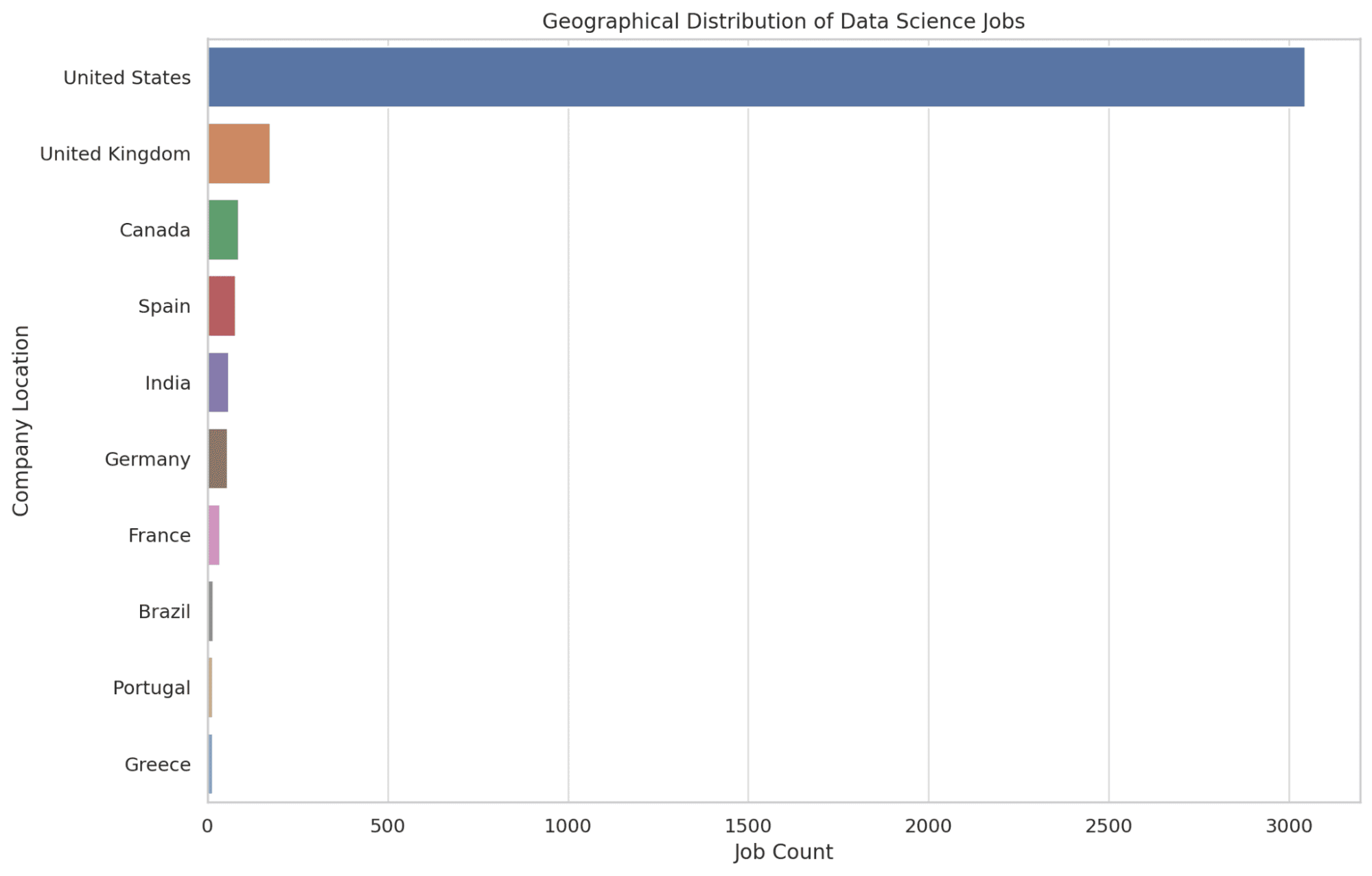
4. Where are Data Science Jobs Primarily Located Geographically?
Here, we pinpoint the top 10 locations holding the highest number of data science job opportunities. We use the COUNT function to determine the number of job postings in each location, arranging them in descending order to spotlight the areas with the most opportunities.
Having this information equips readers with knowledge of the geographical areas that are hubs for data science roles, aiding in potential relocation decisions. Let’s see the code.
SELECT company_location, COUNT(*) AS job_count
FROM salary_data
GROUP BY company_location
ORDER BY job_count DESC
LIMIT 10;
Now let’s create graphs of the code above, with Python.
plt.figure(figsize=(12, 8))
sns.countplot(y='company_location', data=df, order=df['company_location'].value_counts().index[:10])
plt.title('Geographical Distribution of Data Science Jobs')
plt.xlabel('Job Count')
plt.ylabel('Company Location')
graphs.append(plt.gcf())
plt.show()
Let’s see the graph below.
5. Which Job Titles Offer the Top Salaries in Data Science?
Here, we are identifying the top 10 highest-paying job titles in the data science sector. By using the AVG, we calculate the average salary for each job title, sorting them in descending order based on the average salary to highlight the most lucrative positions.
You can aspire to in your career journey, by looking at this data. Let’s proceed to understand how readers can create a Python visualization for this data.
SELECT job_title, AVG(salary_in_usd) AS avg_salary
FROM salary_data
GROUP BY job_title
ORDER BY avg_salary DESC
LIMIT 10;
Here is the output.
(Here we can not use photos, because we added 4 photos above, and one left for a thumbnail, Do we have a chance to use a table like below to demonstrate the output?)
| Rank | Job Title | Average Salary (USD) |
| 1 | Data Science Tech Lead | 375,000.00 |
| 2 | Cloud Data Architect | 250,000.00 |
| 3 | Data Lead | 212,500.00 |
| 4 | Data Analytics Lead | 211,254.50 |
| 5 | Principal Data Scientist | 198,171.13 |
| 6 | Director of Data Science | 195,140.73 |
| 7 | Principal Data Engineer | 192,500.00 |
| 8 | Machine Learning Software Engineer | 192,420.00 |
| 9 | Data Science Manager | 191,278.78 |
| 10 | Applied Scientist | 190,264.48 |
This time, let’s try to create a graph by yourself.
Tips: You can use the following prompt in ChatGPT to generate a Pythonic code of this graph:
<SQL Query here>

Create a Python graph to visualize the top 10 highest-paying job titles in Data Science, similar to the insights gathered from the given SQL query above.
Final Thoughts
As we wrap up our journey through the diverse terrains of the data science career world, we hope SQL proves to be a trustworthy guide, helping you unearth gems of insights to support your career decisions.
I hope that you feel more equipped now, not just in mapping your career path, but also in using SQL in shaping raw data into powerful narratives. So here's to stepping into a future filled with opportunities, with data as your compass and SQL as your guiding force!
Thanks for reading!
Nate Rosidi is a data scientist and in product strategy. He's also an adjunct professor teaching analytics, and is the founder of StrataScratch, a platform helping data scientists prepare for their interviews with real interview questions from top companies. Connect with him on Twitter: StrataScratch or LinkedIn.