Data Analytics Models in Quantitative Finance and Risk Management
We review how key data science algorithms, such as regression, feature selection, and Monte Carlo, are used in financial instrument pricing and risk management.
By Elena Sharova.
Introduction
In this article I would like to go over how some of the data science algorithms are used in financial instrument pricing and risk management. This is a high-level introductory overview, with pointers to resources for more details.
Linear Regression
According to the September KDnuggets poll, regression was voted as the most used algorithm. This is no surprise, since regression is one of the most transparent models. The term ‘regression’ can mean deriving a numeric prediction. Here, by regression I mean the ordinary least-squares regression.
Many financial models rely on historical data, like prices, to forecast the future. Sometimes price data may not be available for a required historical horizon. This is when missing time-series can be modeled using available data, like indices (e.g. S&P 500). The idea here is that systemic risk can be captured with some relevant liquid index and specific risk can be modeled separately, often using other proxies. This modelling set-up is suitable for regression.
Capitalization is important in financial risk management. Investment firms are required to hold capital to ensure solvency. The amount of capital that must be held is often calculated by risk models. Institutions must ensure that the models work, and this is achieved by a model validation function. In the previous paragraph I mentioned how regression can be used to model historical prices. The goodness of fit can be back-tested using regression as well [1]. An analyst may suspect that the price-forecasting regression model is failing to capture true market volatility. If this is the case, then the number of model back-testing exceptions could be explained by spikes in one or more volatility indices, like Vix. Then the regression model for the number of back-testing exceptions over a time-period takes the form:

Where It is the total number of exceptions at time t, β0 is a small acceptable number of exceptions at some confidence level, and betas are the weighted market volatility indices. Figure 1 shows a possible scenario where the back-testing exceptions can be explained by Vix volatility index. The back-test would begin with a null hypothesis that β1 through βk are zero, and a hypothesis test will either support or reject it.
There are many other uses of regression in finance, such as in optimal portfolio allocation, forecasting realized variance and cross-sectional regression [see 2].
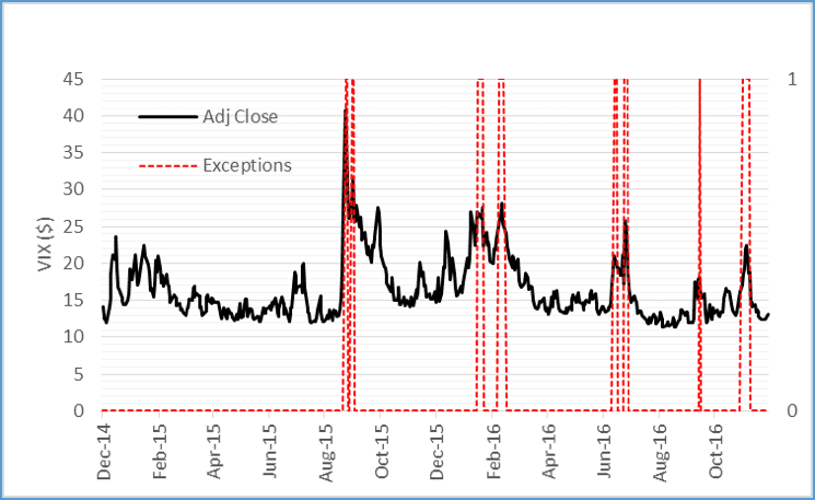
Figure 1. Exceptions (red) and Vix prices (black).
Features Selection
Feature selection is an important part of predictive modelling. Features compression is often done using Principle Component Analysis (PCA). PCA is widely used in quantitative finance.
An investment portfolio of bonds with future cash flows is sensitive to changes in interest rates for different maturities. If we desire to estimate portfolio risk using a smaller number of factors we can use PCA. By performing PCA on historical interest rate moves for the relevant set of maturities, one can select the first n factors explaining most of the variation in the data (see [1], chapter 2, where PCA is performed using a covariance matrix of short rate moves).
Another example is in foreign exchange. The pricing and risk management of foreign exchange derivatives uses volatility surface. A volatility surface of a currency pair shows how implied volatilities vary by moneyness/profitability and maturities. A good example of using PCA in financial risk is to reduce a volatility surface structure in the maturity dimension to a single factor that is most responsible for variation in profit and loss. Value-at-risk is a form of market risk capitalization. One popular method for computing the value-at-risk is through revaluation of a portfolio under a set of moves in price and volatility. When dealing with derivatives that are so-called ‘path dependent’ (e.g. Asian options) one needs to consider entire volatility term structure as opposed to a volatility at a single tenor. However, applying moves to all volatilities is computationally expensive. One solution is to use the output of PCA to reduce the term-structure.
Parametric Modelling and Monte Carlo
Monte Carlo (MC) methods are widely used in machine learning. Take for example generating proposal distributions or simulating experiences to learn optimal policy in reinforcement learning. MC is used extensively in quantitative finance. Pricing financial derivatives can be broadly split into finding expectations analytically or via a simulation. The simulation is often done using MC. The dynamics of the underlying is assumed to follow a stochastic process, like Geometric Brownian Motion. The simulated prices become inputs into a payoff function, and the average discounted payoff determines the price of the derivative. See [3] for an excellent source on this subject.
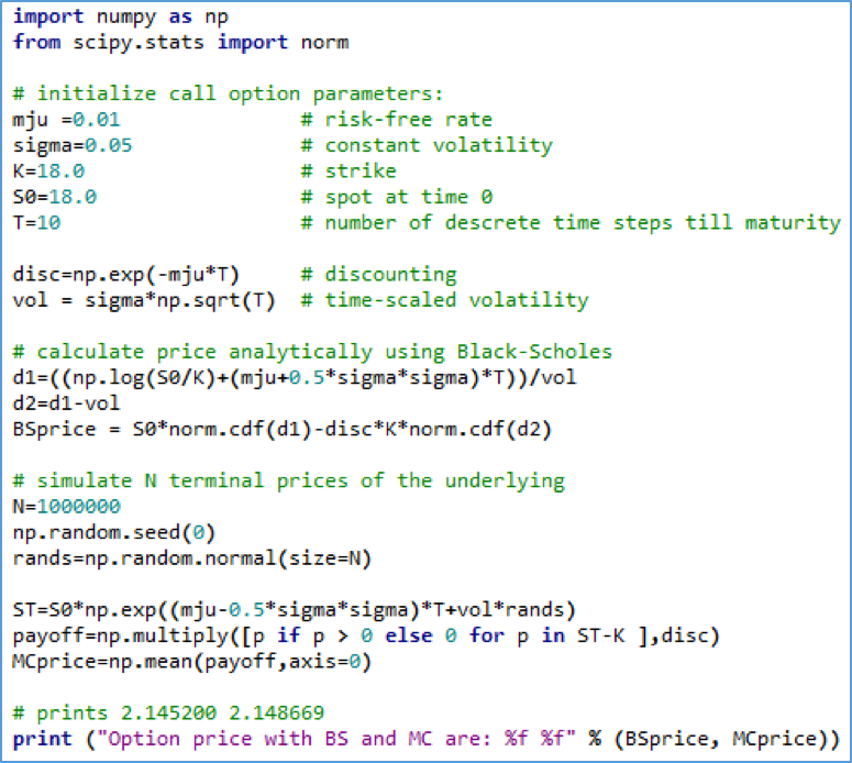
Figure 2. Example Python implementation of pricing a call option on a simple underlying like stock using Black-Scholes and Monte Carlo simulation of terminal price.
In risk, modelling value-at-risk can be broadly split into methods that use historical data to calculate market moves or use some form of parametric approximation to the price moves distribution. MC can be used to simulate such distribution.
Another important use of MC simulation can be found in counterparty credit risk measurement. Instrument prices within a portfolio are simulated until contract maturities. Potential future exposure is a possible loss at a given confidence level due to counterparty default. See [4] as a great source on this topic.
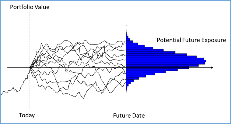
Figure 3. Illustration of potential future exposure calculation.
New Frontiers
The given here examples are barely scratching the surface of the amount of modelling overlap between the two fields; historical and simulation-based probabilistic modelling is at the heart of both.
The management of operational and compliance risks are fast growing areas where quantitative tools are finding new application. Robust machine learning and data science models are helping financial institutions to better understand the nature of operational losses and ensure compliance with regulations. Methods for anomaly detection, pattern recognition and language processing are being used and relied upon.
References:
[1] Carol Alexander, Market Risk Analysis, Value-at-Risk Models (volume 4). John Wiley&Sons, Ltd. 2008.
[2] John Y. Campbell et al, The Econometrics of Financial Markets, Princeton University Press, 1997.
[3] Paul Glasserman, Monte Carlo Methods in Financial Engineering, Springer, 2004.
[4] Jon Gregory. Counterparty Credit Risk, The New Challenge for Global Financial Markets. John Wiley&Sons, Ltd. 2010.
Bio:  Elena Sharova is a data scientist, financial risk analyst and software developer. She holds an MSc in Machine Learning and Data Mining from University of Bristol.
Related: