 Applying Deep Learning to Real-world Problems
 Applying Deep Learning to Real-world Problems
In this blog post I shared three learnings that are important to us at Merantix when applying deep learning to real-world problems. I hope that these ideas are helpful for other people who plan to use deep learning in their business.
By Rasmus Rothe, Co-founder at Merantix.
The rise of artificial intelligence in recent years is grounded in the success of deep learning. Three major drivers caused the breakthrough of (deep) neural networks: the availability of huge amounts of training data, powerful computational infrastructure, and advances in academia. Thereby deep learning systems start to outperform not only classical methods, but also human benchmarks in various tasks like image classification or face recognition. This creates the potential for many disruptive new businesses leveraging deep learning to solve real-world problems.
At Berlin-based Merantix, we work on these new business cases in various industries (currently automotive, health, financial and advertising).
Academia often differs from the real world (source: mimiandeunice.com).
It easier than ever before to train a neural network. However, it is rarely the case that you can just take code from a tutorial and directly make it work for your application. Interestingly, many of the most important tweaks are barely discussed in the academic literature but at the same time critical to make your product work.

Applying deep learning to real-world problems can be messy (source: pinsdaddy.com).
Therefore I thought it would be helpful for other people who plan to use deep learning in their business to understand some of these tweaks and tricks.
In this blog post I want to share three key learnings, which helped us at Merantix when applying deep learning to real-world problems:
- Learning I: the value of pre-training
- Learning II: caveats of real-world label distributions
- Learning III: understanding black box models
A little disclaimer:
- This is not a complete list and there are many other important tweaks.
- Most of these learnings apply not only to deep learning but also to other machine learning algorithms.
- All the learnings are industry-agnostic.
- Most of the ideas in the post refer to supervised learning problems.
This post is based on my talk I gave on May 10 at the Berlin.AI meetup (the slides are here).
Learning I: the value of pre-training
In the academic world of machine learning, there is little focus on obtaining datasets. Instead, it is even the opposite: in order to compare deep learning techniques with other approaches and ensure that one method outperforms others, the standard procedure is to measure the performance on a standard dataset with the same evaluation procedure. However, in real-world scenarios, it is less about showing that your new algorithm squeezes out an extra 1% in performance compared to another method. Instead it is about building a robust system which solves the required task with sufficient accuracy. As for all machine learning systems, this requires labeled training from which the algorithm can learn from.
For many real-world problems it is unfortunately rather expensive to get well-labeled training data. To elaborate on this issue, let’s consider two cases:
- Medical vision: if we want to build a system which detects lymph nodes in the human body in Computed Tomography (CT) images, we need annotated images where the lymph node is labeled. This is a rather time consuming task, as the images are in 3D and it is required to recognize very small structures. Assuming that a radiologist earns 100$/h and can carefully annotate 4 images per hour, this implies that we incur costs of 25$ per image or 250k$ for 10000 labeled images. Considering that we require several physicians to label the same image to ensure close to 100% diagnosis correctness, acquiring a dataset for the given medical task would easily exceed those 250k$.
- Credit scoring: if we want to build a system that makes credit decisions, we need to know who is likely to default so we can train a machine learning system to recognize them beforehand. Unfortunately, you only know for sure if somebody defaults when it happens. Thus a naive strategy would be to give loans of say 10k$ to everyone. However, this means that every person that defaults will cost us 10k$. This puts a very expensive price tag on each labeled datapoint.
Obviously there are tricks to lower these costs, but the overall message is that labeled data for real-world problems can be expensive to obtain.
How can we overcome this problem?
Pre-training

Pre-training helps (source: massivejoes.com).
The basic idea of pre-training is that we first train a neural network (or another machine learning algorithm) on a cheap and large dataset in a related domain or on noisy data in the same domain. Even though this will not directly solve the original problem, it will give the neural network a rough idea of what your prediction problem looks like. Now, in a second step, the parameters of the neural network are further optimized on a much smaller and expensive dataset of the problem you are actually trying to solve. This two-step procedure is depicted in the figure below.
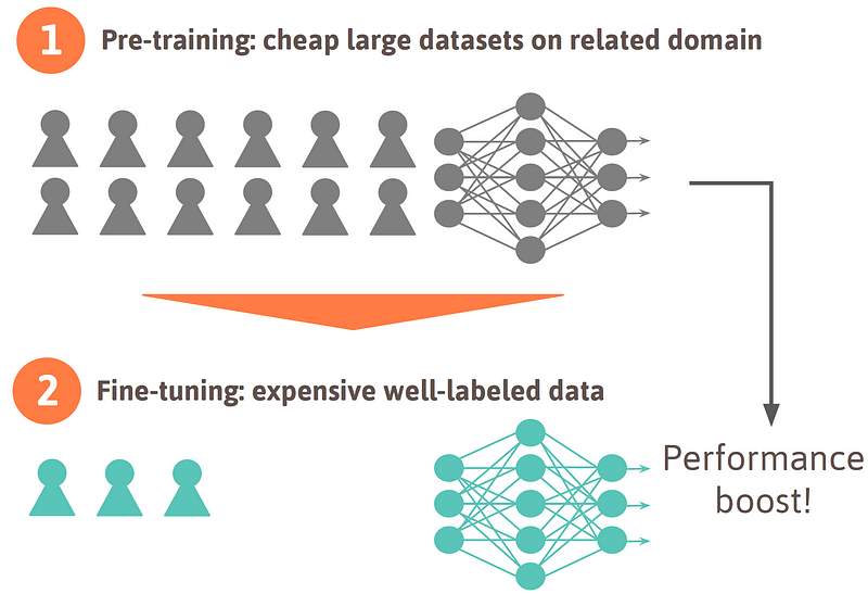
When training data is hard to get: first pre-train the neural network on a large and cheap dataset in a related domain; secondly, fine-tune it on an expensive well-labeled dataset. This will result in a performance boost compared to just training on the small dataset.
When fine-tuning, the number of classes might change: people often pre-train a neural network on a dataset like ImageNet with 1000 classes and then fine-tune it to their specific problem which likely has a different number of classes. This means the last layer needs to be re-initialized. The learning rate is then often set a bit higher on the last layer as it needs to be learned from scratch, whereas the previous layers are trained with a lower learning rate. For some datasets like ImageNet the features (the last fully connected layer) learned are so generic that they can be taken off-the-shelfand directly be used for some other computer vision problem.
How do we obtain data for pre-training?
Sources of data for pre-training
- Pre-trained models: there are lots of trained models on the web. The first go to point are the so-called Model Zoos. These are websites which contain a collection of various trained models by academics, companies and deep learning enthusiasts. See here, here, or here.
- Public datasets: there are many datasets out there on the web. So don’t waste time on collecting the dataset yourself, but rather check if there is already something out there that might help solving the particular problem you’re working on. See here, here, or here.
- Data crawling: if there is neither a public pre-trained model nor dataset, there might be a cheeky way to generate a dataset without labeling it by hand. You can build a so-called crawler which automatically collects them from specific websites. This way you create a new dataset.
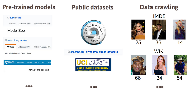
Sources of data for pre-training.
Weakly labeled data
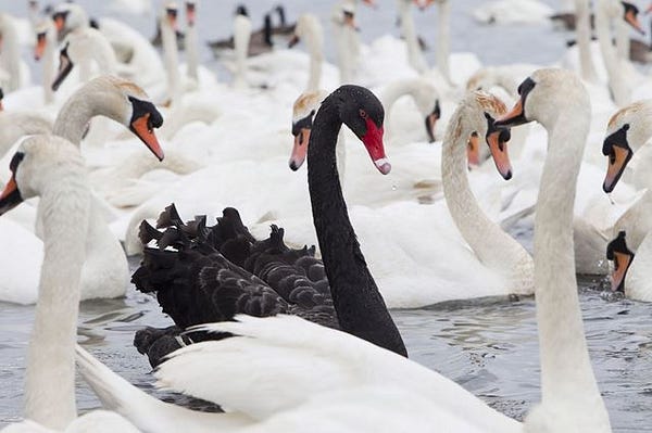
As we fine-tune on precisely labeled data, it is possible to pre-train on so-called weakly labeled data. By this we refer to data which labels are not in all cases correct (i.e. 90% of the labels might be correct and 10% wrong). The advantage is that this kind of data can often be obtained without any human involved in labeling but automatically. This makes this data relatively cheap compared to data where a human needs to label every single image. To give an example: during my PhD, I crawled a dataset of 500k face imagesfrom Wikipedia and IMDb. We combine the date of birth of a person in the profile and any hint in the caption of the photos when it was taken. This way we can assign an approximate age to each image. Note that in some cases the year in the caption below the image might have been wrong or the photo might show several people and the face detector selected the wrong face. Thus we cannot guarantee that in all cases the age label is correct. Nonetheless we showed that pre-training on this weakly labeled dataset helped to improve the performance versus just training on a precisely labeled smaller dataset.
A similar logic can be applied to the medical vision problem where it is required to have several doctors independently label the same image in order to be close to 100% sure that the labeling is correct. This is the dataset for fine-tuning. Additionally, one can collect a larger dataset with weak labels which was annotated by just one person. Thereby, we can reduce the total cost for labeling and still make sure that the neural network has been trained on a diverse set of images.
In summary, increasing performance doesn’t necessarily mean that you need human annotations which are often expensive but you might be able to get a labeled dataset for free or at substantially lower costs.
Learning II: caveats of real-world label distributions
Real-world distributions (source: r4risk.com.au).
Now that we have obtained data both for pre- and fine-tuning, we can move on and start training our neural networks. Here comes another big difference between academia and real world.
In academia, the datasets are mostly balanced. That means for supervised classification problems there are usually equally many samples per class. Below you find two examples: MNIST is a very known dataset of handwritten digits containing approximately equally many samples of each digit. Food 101 is another example of an academic dataset which contains exactly 1000 images of each of the 101 food categories.
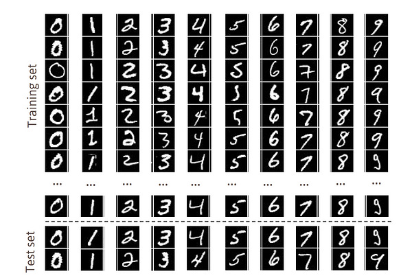

MNIST and Food101 are both balanced datasets.
Unbalanced label distribution
Again I want to illustrate that problem by emphasizing two real-world examples:
- Medical vision: training data for medical imaging is very skewed. The majority of patients are healthy, while only a small fraction of the patients suffer from a certain disease.
- Credit scoring: in fact, the majority of customers returns the loan while only 1–2% of people defaults.
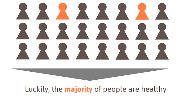
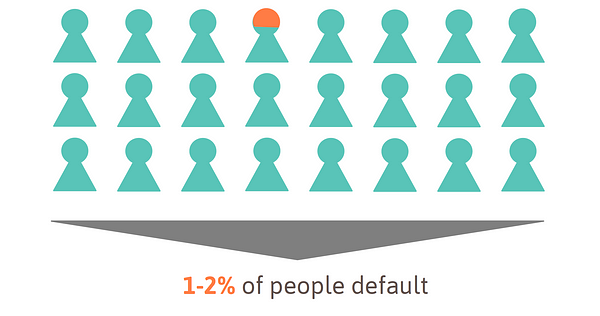
Unbalanced real-world label-distributions.
As illustrated above, the distributions of labels are very skewed in those two cases. This is typical for most real-world applications. Actually, it is very rare that there are equally many samples of each category.
Unbalanced cost of misclassification
Unfortunately, it gets even worse: in academic datasets, the cost of misclassification is usually the same for each class. This is again very different in many real-world applications:
- Medical vision: diagnosing somebody as sick who is healthy is not that bad if the doctor double-checks and then realizes that the person is actually healthy. However, not identifying a patient who is sick and then letting him go without any treatment is very dangerous.
- Credit scoring: reject a loan for somebody who would have paid back is not bad, as it means that you would only lose out on the interest. However, giving a loan to somebody who defaults is very expensive, as you will have to cover the cost for the entire loan.
This is illustrated in the figure below.
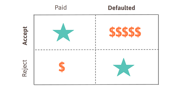
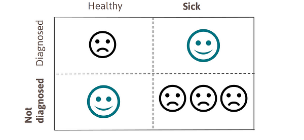
Imbalanced cost of misclassification for real-world applications.
How to cope with this issue?
After having realized that the classes are often not balanced and the cost for misclassification is neither, we need to come up with techniques to cope with that. The literature covering this topic is rather limited, and one mostly finds blog posts and Stack Overflow questions touching some of the ideas.
Note that both the imbalanced classes and the cost of misclassification are highly related, as it means that for some of the samples we have not only little training data, but also making mistakes is even more expensive.
I grouped the techniques which help to make our model especially good at classifying these rare examples into four categories:
1. More data
The obvious approach is to try to collect more data from the rare classes. For the medical vision example, this implies that we try to focus on collecting images of patients who have a certain disease we try to diagnose. If this is not possible because it is too expensive, there might be other ways to obtain training data, as mentioned in the previous section. Note that you have to be careful when adjusting the distribution of training labels, as this will have an impact on the way the model predicts at inference: if you increase the number of sick patients in your training set, the model will also predict sickness more often.
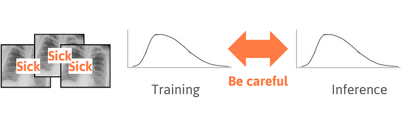
Collecting more data of rare classes. Be careful when the distribution of labels during training and inference do not match.
2. Change labeling
If you cannot get more data of the rare classes another approach is to rethink the taxonomy. For the practical application it might not be needed to differentiate between disease A or B as long as you recognize that it’s either of the two. In that case you can just join the two classes. Either already at training time to simplify the training procedure, or during inference, which means you do not penalize if disease A or B get confused.
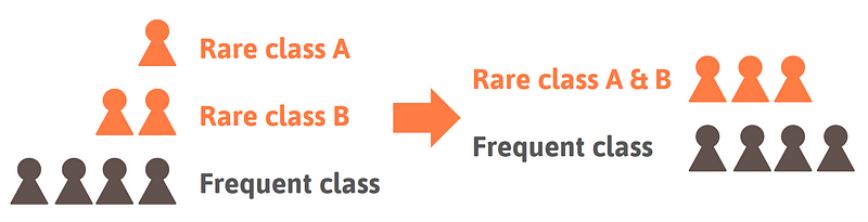
Merging two or more classes during training or evaluation can simplify the problem.
3. Sampling
If you can neither get more data nor change the labeling, this means you need to work with the original data. How can you still make sure that the model gets especially good at the rare classes? You just change the way the algorithm sees the examples during training. Normally, the samples are just uniformly sampled. This means the algorithm sees each example equally likely during training.
There are a few different sampling methods which help to improve the performance of the label for some rare class.
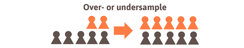
- Ignore. Ignoring some samples of the more frequent class is probably the simplest method. This can be done up to the point at which there are (roughly) equally many samples from each class.

- Over- or undersample. Oversampling means that samples from the rare class are shown to the algorithm with higher frequency whereas undersampling refers to the opposite: the samples of the more frequent class are shown less. From the perspective of the algorithm, both methods lead to the same result. The advantage of this technique compared to the previous is that no samples are ignored.
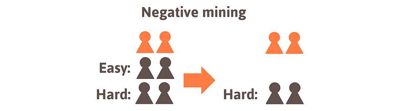
- Negative mining. The third group of sampling methods is a bit more complex but indeed the most powerful one. Instead of over- or undersampling, we choose the samples intentionally. Although we have much more samples of the frequent class we care most about the most difficult samples, i.e. the samples which are misclassified with the highest probabilities. Thus, we can regularly evaluate the model during training and investigate the samples to identify those that are misclassified more likely. This enables us to wisely select the samples that are shown to the algorithm more often.
4. Weighting the loss
By applying the methods 1–3 described within this section, we have done everything to our data in terms of improving the class distribution. Therefore, we can now shift our focus towards the algorithm itself. Luckily, there are methods that can be applied during training in order to put more attention to rare classes. A very straightforward way is to increase the weight of the loss of samples from rare classes.
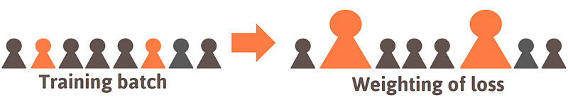
The loss of the rare classes is weighted more.
Learning III: understanding black box models

A black box (source: The Simpsons).
As mentioned already in the section about pre-training, the most important goal in academia is to reach or outperform state-of-the-art performance, no matter what the model is like. When working on real-world applications it is often not enough to just design a model that performs well.
Instead, it is important to be able to
- understand why and how a model can make wrong predictions,
- give some intuition why our model can perform better than any previous solution,
- make sure that the model cannot be tricked.
Before the rise of deep neural networks, most models were relatively easy to reason about. Consider the following:
- Linear models: linear classifiers or regressors valuably provide a direct relationship between each feature and the prediction. This makes it relatively straightforward to reason about the decision mechanism of the model.
- Decision trees: the beauty about decision trees lies in the fact that one can just follow down the tree to understand how the decision was formed. Generally, the top nodes cover the most important features. It gets a bit more difficult when talking about random decision forests, nonetheless the tree structure allows relatively good reasoning.
Unfortunately, it is much more difficult to understand the decision mechanism of deep neural networks. They are highly non-linear and can easily have more than 100 million parameters. This makes it difficult to come up with a simple explanation of how a decision is formed.
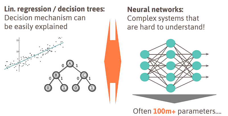
Comparison of classical machine learning methods vs deep learning.
This becomes an important challenge in real-world applications as deep neural networks are rapidly entering many areas of our lives: autonomous driving, medical diagnostics, financial decision-making, and many more. Most of these applications directly lead to outcomes that significantly affect our lives, assets or sensitive information. Therefore, wrong decisions by algorithms can hurt people or cause financial damage.
The Tesla accident (left) and an article about AI turning racist (right).
Unfortunately, these failures could not only happen by accident but also be caused by attackers. To demonstrate the relevance of this topic, research has shown that by adding just simple random noise to a normal image, the classification result of a deep neural network can be changed (left figure) while the image appears to be unchanged to any human. Similarly it is possible to fit in completely artificial images and still receive a very confident prediction (right figure).
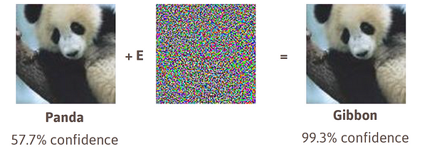
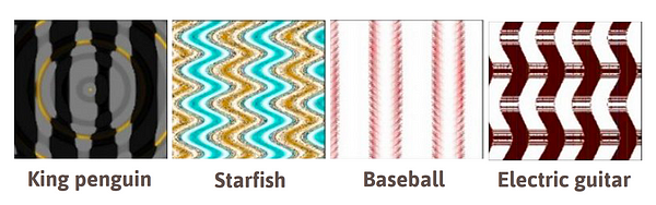
Adding little random noise to an image (left) or even completely artificial images (right) can easily fool neural networks.
In real life, generally, you want to understand the reason why your system doesn’t behave as it should.
At Merantix, we take these problems very seriously and believe that they will become even more important in the future, as more deep learning systems will be used in critical real-world applications.
Recently we open-sourced a deep learning visualization toolbox called Picasso (Medium Post, Github). As we work with a variety of neural network architectures, we developed Picasso to make it easy to see standard visualizations across our models in our various verticals: including applications in automotive, e.g. to understand when road segmentation or object detection fail; advertisement, such as understanding why certain creatives receive higher click-through rates; and medical imaging, such as analyzing what regions in a CT or X-ray image contain irregularities. Below I have included a demo of our open-source Picasso visualizer.

Picasso visualizer demo.
Conclusion
In this blog post I shared three learnings that are important to us at Merantix when applying deep learning to real-world problems. I hope that these ideas are helpful for other people who plan to use deep learning in their business. As mentioned in the beginning, there are many more tweaks, tricks and learnings (cascading models, smart augmentation, sensible evaluation metrics, building reusable training pipelines, efficient inference and reducing model size, etc.) when making deep learning work for real-world applications. Please feel free to reach out if you would like to discuss some of the tweaks or a specific application of deep learning.
Acknowledgments
- Jonas for helping with the illustrations.
- Hanns, Bosse, Matthias, Jonas, Stefan, Katja and Adrian for reviewing and discussion of this article.
Bio: Rasmus Rothe is one of Europe's leading experts in deep learning and a co-founder at Merantix. He studied Computer Science with a focus on deep learning at ETH Zurich, Oxford, and Princeton. Previously he launched howhot.io as part of his PhD research, started Europe's largest Hackathon HackZurich and worked for Google and BCG.
Original. Reposted with permission.
Related: