Urban Sound Classification with Neural Networks in Tensorflow
This post discuss techniques of feature extraction from sound in Python using open source library Librosa and implements a Neural Network in Tensorflow to categories urban sounds, including car horns, children playing, dogs bark, and more.
By Aaqib Saeed, University of Twente.
We all got exposed to different sounds every day. Like, the sound of car horns, siren and music etc. How about teaching computer to classify such sounds automatically into categories!
In this blog post, we will learn techniques to classify urban sounds into categories using machine learning. Earlier blog posts covered classification problems where data can be easily expressed in vector form. For example, in the textual dataset, each word in the corpus becomes feature and tf-idf score becomes its value. Likewise, in anomaly detection dataset we saw two features “throughput” and “latency” that fed into a classifier. But when it comes to sound, feature extraction is not quite straightforward. Today, we will first see what features can be extracted from sound data and how easy it is to extract such features in Python using open source library called Librosa.
To get started with this tutorial, please make sure you have following tools installed:
- Tensorflow
- Librosa
- Numpy
- Matplotlib
Dataset
We need a labelled dataset that we can feed into machine learning algorithm. Fortunately, some researchers published urban sound dataset. It contains 8,732 labelled sound clips (4 seconds each) from ten classes: air conditioner, car horn, children playing, dog bark, drilling, engine idling, gunshot, jackhammer, siren, and street music. The dataset by default is divided into 10-folds. To get the dataset please visit the following link and if you want to use this dataset in your research kindly don’t forget to acknowledge. In this dataset, the sound files are in .wav format but if you have files in another format such as .mp3, then it’s good to convert them into .wav format. It’s because .mp3 is lossy music compression technique, check this link for more information. To keep things simple, we will use sound files from only one fold.
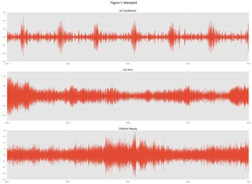
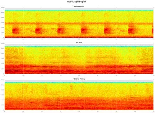
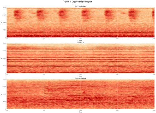
Let’s read some sound files and visualise to understand how different each sound clip is from other. Matplotlib’s specgram method performs all the required calculation and plotting of the spectrum. Likewise, Librosa provide handy method for wave and log power spectrogram plotting. By looking at the plots shown in Figure 1, 2 and 3, we can see apparent differences between sound clips of different classes.