 The Anatomy of Deep Learning Frameworks
 The Anatomy of Deep Learning Frameworks
This post sketches out some common principles which would help you better understand deep learning frameworks, and provides a guide on how to implement your own deep learning framework as well.
Gokula Krishnan Santhanam, ETH Zurich.
Deep Learning, whether you like it or not is here to stay, and with any tech gold-rush comes a plethora of options that can seem daunting to newcomers.
If you were to start off with deep learning, one of the first questions to ask is, which framework to learn? I’d say instead of a simple trial-and-error, if you try to understand the building blocks of all these frameworks, it would help you make an informed decision. Common choices include Theano, TensorFlow, Torch, and Keras. All of these choices have their own pros and cons and have their own way of doing things. After exploring the white papers and the dev docs, I could understand the design choices and was able to abstract the fundamental concepts that are common to all of these.
In this post, I have tried to sketch out these common principles which would help you better understand the frameworks and for the brave hearts among you, provide a guide on how to implement your own deep learning framework. The interesting thing about these principles is that they are not specific to DL alone, they are applicable whenever you want to do a series of computations on data. Hence, most DL frameworks can be used for non-DL tasks as well (see www.tensorflow.org/tutorials/mandelbrot/)
There are a few core components of a DL framework, these are:
- A Tensor Object
- Operations on the Tensor Object
- A Computation Graph and Optimizations
- Auto-differentiation tools
- BLAS / cuBLAS and cuDNN extensions
These should make your framework complete, but you would need to polish it to make it more easy to use. I will be using references to the Python NumPy package in this article to make it easier to understand. If you haven’t used NumPy before, fret not, this article should be easy to understand even if you skip the numpy parts. I’m a believer of understanding a system at multiple levels of abstractions so you will be seeing discussions of low-level optimizations interspersed with high-level Calculus and Linear Algebra. Drop a comment below if something needs more explanation!
NOTE: I have been a contributor to Theano and hence might be biased towards it in citing references. Having said that, theano also has one of the most informative websites of all the frameworks I’ve come across.
A Tensor Object
At the heart of the framework is the tensor object. A tensor is a generalization of a matrix to n-dimensions (think numpy’s ndarrays). In other words, a matrix is a two-dimensional tensor with (rows, columns). An easy way to understand tensors is to consider them as N-D Arrays.
As an example, take a color image. Let’s say it’s an RGB Bitmap image of size 258 x 320 (Height x Width). This is a three-dimensional tensor (height, width, channels). Take a look at the following images to understand this better (taken from: github.com/parambharat/CarND-helpers/blob/master/image_processing/Image_processing_tutorial.ipynb)
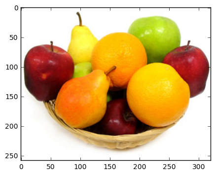
A Normal RGB Image
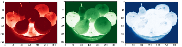
Red, Green and Blue Channels of the same image
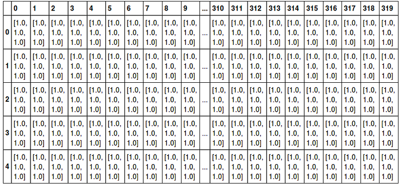
The same image represented as a 3D Tensor
As an extension, a set of 100 images can be represented as a 4D tensor (ID of image, height, width, channels).
Similarly, we represent all input data as tensors¹ before feeding them into the neural net. This is an abstraction necessary before we can feed data into a net, else we would have to define operations that work on each type and that’s a lot of wasted effort². We would also need to be able to get back data in a form we want.
So, we need a Tensor Object that supports storing the data in form of tensors. Not just that, we would like the object to be able to convert other data types (images, text, video) into tensors and back. Think of something like numpy.imread and numpy.imsave, they read images as ndarrays and store ndarrays as images respectively.
The basic Tensor object needs to support representing data in form of a tensor. This means supporting indexing, overloading operators, having a space efficient way to store the data and so on. Depending on further design choices, you might have to add more features as well.
Operations on the Tensor Object
A neural network can be considered as a series of Operations performed on an input tensor to give an output. Learning is done by correcting the errors between the output created by the net and the expected output³. These operations could be something simple like matrix multiplication (in sigmoids) or more complicated like convolutions, pooling or LSTMs.
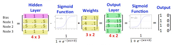
Sigmoid layer represented as Matrix Operations, from www.datasciencecentral.com/profiles/blogs/matrix-multiplication-in-neural-networks
Check out the following links to get an idea of how extensive these operations could be:
- NumPy: www.scipy-lectures.org/intro/numpy/operations.html
- Theano: deeplearning.net/software/theano/library/tensor/basic.html
- TensorFlow: www.tensorflow.org/api_docs/python/math_ops/
You could just skip this part and ask the user to implement these operations themselves, but it is too cumbersome and outright inefficient. Moreover, most operations are common enough that one could justify making them a part of the framework to spare headaches for the users. NumPy does a pretty good job of having a lot of operations already implemented (it’s insanely fast as well) and there is a running theano issue about incorporating more operations which show how important it is to have more operation supported by the framework.
Instead of implementing operations as functions, they are usually implemented as classes. This allows us to store more information about the operation like calculated shape of the output (useful for sanity checks), how to compute the gradient or the gradient itself (for the auto-differentiation), have ways to be able to decide whether to compute the op on GPU or CPU⁴ and so on. Again, this idea is similar to classes used for various algorithms implemented by scikit-learn. You could define a method called compute that does the actual computation and returns the tensor after the computation is done.
These classes are usually derived from an abstract class (in theano, it’s the Op class). This enforces a unified interface across the Ops and also provide a way to add new ops later on. This makes the framework very flexible and ensures people can use it even as new network architectures and nonlinearities come along.
Computation Graph and Optimizations
So far, we have classes for representing tensors and operations on them. The power of neural networks lies in the ability to chain multiple such operations to form a powerful approximator.
Therefore, the standard use case is that you can initialize a tensor, perform actions after actions on them and finally interpret the resulting tensor as labels or real values. Sounds simple enough?
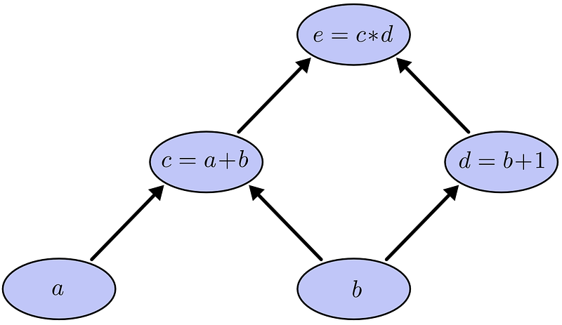
Chaining together different operations, taken from colah.github.io/posts/2015-08-Backprop/
Unfortunately, as you chain more and more operations together, several issues arise that can drastically slow down your code and introduce bugs as well.
- Start later ops only after the previous one is done or do them in parallel?
- How to assign to different devices and coordinate between them?
- How do you avoid redundant operations (multiplying with ones, adding zeros), cache useful intermediate values, and reduce multiple operations into one ( replace mul(mul(mul(Tensor,2),2),2) with one mul(Tensor, 8) )
There are more such issues and it becomes necessary to be able to get a bigger picture to even notice that these issues exist. We need a way to optimize the resultant chain of operations for both space and time.
In order to get a bigger picture, we introduce a Computation Graph which is basically an object that contains links to the instances of various Ops and the relations between which operation takes the output of which operation as well as additional information. Depending on the framework in question, this can be implemented in different ways.
For example,
- Theano deeplearning.net/software/theano/extending/graphstructures.html
- TensorFlow download.tensorflow.org/paper/whitepaper2015.pdf
- Caffe http://caffe.berkeleyvision.org/tutorial/net_layer_blob.html
Like many ideas in Deep Learning, the idea of computation graphs has been around for quite some time. Take a look at any Compilers textbook and you can find similar ideas in Abstract Syntax Trees and Intermediate Representations used for Optimization. These ideas have been extended and adapted to the Deep Learning scenario to give us the computational graph. The idea of optimizing the graph before code generation (will be covered later) is straightforward. The optimizations themselves could again be implemented as classes or functions⁵ and could be selectively applied depending on whether you want the code to compile fast or run fast⁶.
Additionally, since you get a bird’s eye view of what will be happening in the network, the graph class can then decide on how to allocate GPU memory (like Register Allocation in Compilers) and coordinate between various machines when deployed in a distributed environment. This helps us to effectively solve the three problems mentioned above.
Auto-differentiation tools
Another benefit of having the computational graph is that calculating gradients used in the learning phase becomes modular and straightforward to compute. This is thanks to the chain rule⁷ that lets you calculate derivatives of composition of functions in a systematic way. As we saw earlier, neural nets can be thought of composition of simple nonlinearities giving rise to more complex functions. Differentiating these functions is simply traversing the graph from the outputs back to the inputs⁸. Symbolic Differentiation or Automatic Differentiation⁹ is a programmatic way by which gradients can be computed in a computation graph.
Symbolic differentiation refers to calculating the derivatives analytically i.e., you get an expression of what the gradient is. To use it, you simply plug in the values into the derivative and use it. Unfortunately, some nonlinearities like ReLU (Rectified Linear Units) are not differentiable at some points. So, we instead calculate the gradient in an iterative manner. Since the second method could be used universally, most computational graph packages like Computation Graph Toolkit (rll.berkeley.edu/cgt/) implement auto-differentiation but you can use symbolic differentiation if you are creating your own.
It is usually not a good idea to roll out your own gradient computation module because it is easier and faster for the toolkit to provide it as part of the package. So, either have your own Computation Graph toolkit and auto-differentiation module or use an external package for both.
Since the derivative at each node has to computed with respect to only its adjacent nodes, the method to compute gradients can be added to the class¹⁰ ¹¹ and can be invoked by the differentiation module.
BLAS / cuBLAS and cuDNN extensions
With all the above components, you can stop right now and have a fully functional Deep Learning framework. It would be able to take data as input and convert to tensors, perform operations on them in an efficient way, compute gradients to learn and return back results for the test dataset. The problem, however, lies in the fact that since you most likely implemented it in a high-level language (Java / Python / Lua), there is an inherent upper limit to the speedups you can get. This is because even the simplest operations in a high-level language take more time (CPU cycles) than when done in a low-level language.
In these situations, there are two different approaches we could take.
The first one is an another analogy from compilers. The last step of a compilation process is hardware specific code generation in Assembly. Similarly, instead of running the graph written in the high-level language, the corresponding code for the network is generated in C and this is compiled and executed. The code for this is stored in each of the Ops and can be combined together in the compilation phase¹². Transferring data to and from the low-level to high-level code is done by wrappers like pyCUDA and Cython.
The second approach is to have a backend implemented in a low-level language like C++, this means that the low-level language — high-level language interaction is internal to the framework unlike the previous approach and could be faster because we don’t need to compile the entire graph every time. Instead, we could just call the compiled methods with the appropriate arguments¹³.
Another source of non-optimal behavior comes from slow implementations at the low-level language. It is difficult to write efficient code¹⁴ and we will be better off using libraries that have optimized implementations of these methods. BLAS or Basic Linear Algebra Subprograms are a collection of optimized matrix operations, initially written in Fortran¹⁵. These can be leveraged to do very fast matrix (tensor) operations and can provide significant speedups. There are many other software packages like Intel MKL, ATLAS which also perform similar functions. Which one to choose is a personal preference.
BLAS packages are usually optimized assuming that the instructions will be run on a CPU. In the deep learning situation, this is not the case and BLAS may not be able to fully exploit the parallelism offered by GPGPUs. To solve this issue, NVIDIA has released cuBLAS¹⁶ which is optimized for GPUs. This is now included with the CUDA toolkit and is probably why not many people have heard of it. Finally, cuDNN¹⁷ is a library that builds on the featureset of cuBLAS and provides optimized Neural Network specific operations like Winograd Convolution and RNNs.
So, by using these packages, you could gain significant speed-ups in your framework. Speed-ups are important in DL because it is the difference between training a neural network in four hours instead of four days. In the fast moving world of AI startups, that’s the difference between being a pioneer and playing a game of catch-up. So exploit parallelism and optimized libraries wherever you can!
Conclusion
We have finally come to the end of a pretty long post, thanks a lot for reading it. I hope I have demystified the anatomy of deep learning frameworks for many of you. My main goal in writing this post was to make concrete my understanding of how different frameworks are doing essentially the same thing. This will be a very helpful exercise for anyone who’s above a novice level but below a pro level (a semi-pro, if you will). Once you can understand how things work behind the scenes, they become easier to approach and master. Frameworks do a great job in abstracting away most of these ideas in order to provide a simple interface for the programmers. No wonder that most of these concepts are not very evident when you are learning a framework.
As someone who’s interested in not just the applications of Deep Learning but also in the fundamental challenges of the field, I believe that knowing how things work under the hood is an important step towards mastery of the topic as it clears out many of the misunderstandings and provides a simpler way to think about why things are the way they are. I sincerely believe that a good worker knows not just which tool to use but also why that tool is the best choice. This blog is a step in that direction.
Hope you enjoyed reading this post as much as I did writing it. Please do let me know your thoughts in the comments below!
If you found this interesting, and want to know more about me/hire me as an intern, I’d love to hear from you! You can find my CV here.
Footnotes
- [1] It’s not straightforward how you would represent text as tensors. The first way is to use a one-hot encoding, which is a very sparse matrix and wastes a lot of space. A more dense representation is word vectors. These are pretty cool and I probably might write another post on them if enough people are interested!
- [2] Also, as you will see in the Auto-differentiation part, it’s not clear how you would calculate the derivatives of words. They’re not even continuous!
- [3] This is the (in)famous backpropagation algorithm and is central to learning in Multilayered neural networks.
- [4] This also means moving the data to GPU or back. I have noticed that in Theano (possibly other frameworks as well), this is the most time-consuming part during execution.
- [5] http://www.deeplearning.net/software/theano/optimizations.html
- [6]deeplearning.net/software/theano/library/config.html#config.mode
- [7] d(f(g(x)) / dx = (df / dg) * (dg / dx). cf.en.wikipedia.org/wiki/Chain_rule
- [8] Check out https://colah.github.io/posts/2015-08-Backprop/ for a more detailed discussion of derivatives on computational graphs
- [9] https://en.wikipedia.org/wiki/Automatic_differentiation
- [10] https://www.tensorflow.org/how_tos/adding_an_op/
- [11] http://deeplearning.net/software/theano/tutorial/gradients.html
- [12]deeplearning.net/software/theano/extending/extending_theano_c.html#methods-the-c-op-needs-to-define
- [13] Both TensorFlow and Caffe do this.
- [14] If you are interested, you can check out the materials ofwww.inf.ethz.ch/personal/markusp/teaching/263-2300-ETH-spring11/course.html, will be taking this next sem :)
- [15] http://www.netlib.org/blas/
- [16] https://developer.nvidia.com/cublas
- [17] https://developer.nvidia.com/cudnn
Bio: Gokula Krishnan Santhanam is a Masters Student in CS at ETH Zurich, a Deep Learning Researcher, and a Pythonista.
Original. Reposted with permission.
Related: