 Understanding Machine Learning Algorithms
 Understanding Machine Learning Algorithms
Machine learning algorithms aren’t difficult to grasp if you understand the basic concepts. Here, a SAS data scientist describes the foundations for some of today’s popular algorithms.
By Brett Wujek, SAS.
Machine learning is now mainstream. And given the success companies see deriving value from the vast amount of available data, everyone wants in. But while the thought of machine learning can seem overwhelming, it’s not magic, and the basic concepts are fairly simple.
Here I’ll give you a foundation for understanding the ideas behind some of the most popular machine learning algorithms.
Random Forests
Devised by Leo Breiman in 2001, a random forest is a simple, yet powerful algorithm comprised of an ensemble (or collection)of independently trained decision trees.
In a decision tree, the entire data set of observations is recursively partitioned into subsets along different branches so that similar observations are grouped together at the terminal leaves. The variable that optimally increases the “purity” of the tree directs the partitioning at each split point, grouping observations with similar target values. For any new observation, you can follow the path of splitting rules through the tree to predict the target.

But decision trees are unstable. Small changes in training data can lead to wildly different trees. Training a group of trees and “ensembling” them to create a “random forest” model enables more robust prediction.
In a random forest:
- The data set used to train each tree is a random sample of the complete data set (with replacement), a process known as “bagging” (bootstrap aggregating).
- Input variables considered for splitting each node are a random subset of all variables, reducing bias toward the most influential factors and allowing secondary factors to play a role in the model.
- Trees are overfit by letting them grow to a large depth and small leaf size. Averaging the predicted probabilities for a large number of overfit trees is more robust than using a single, fine-tuned decision tree.
Ensembling, or scoring new observations on many trees enables you to obtain a consensus for a predicted target value(voting for classification, averaging for interval target prediction) with a more robust and generalizable model.
Because random forests are so effective, researchers have evolved variants such as “similarity forests” and “deep embedding forests.”
Gradient Boosting Machines
A gradient boosting machine, such as XGBoost, is another machine learning algorithm derived from decision trees.
In the late 90’s, Breiman observed that a model that exhibits a certain level of error can serve as a base learner that can be improved by iteratively adding models that compensate for the error – a process called “boosting.” Each added model is trained to minimize the error by searching in the negative gradient direction (thus “gradient” boosting). Boosting is a sequential process since new models are added based on the results of previous models.
Jerome Friedman applied the gradient boosting concept to decision trees in 2001to create Gradient Boosting Machines. The popular and effective Adaboost from Freund and Shapire (2001), which uses an exponential loss function, is a variant of this approach.

In recent years, Tiangi Chen studied all aspects and revisions of the gradient boosting machine algorithm to further enhance performance in an implementation known as XGBoost, which stands for “extreme gradient boosting.”His modifications included using quantile binning in the decision tree training, adding a regularization term to the objective to improve generalization, and supporting multiple forms of the loss function. Ultimately, the “extreme” nature of XGBoost could be attributed to the fact that Chen implemented it specifically to take advantage of the more readily available computing power with distributed multi-threaded processing for speed and efficiency.
Support Vector Machines
Yet another “machine” in the machine learning practitioner’s toolbox, a support vector machine (SVM), is one that has been around for many decades. Invented in 1963 by Vladimir Vapnik and Alexey Chervonenkis, SVM is a binary classification model that constructs a hyperplane to separate observations into two classes.
The figure below is a simple example with target values for observations represented by dots and x’s, which can split as shown. Since an infinite number of orientations for this line (a hyperplane in multiple dimensions)can separate these points, we define a buffer zone around this line and formulate an optimization problem to maximize this margin. The more we can separate these two classes, the more accurate our model will be when scoring new data. The points that define the margin are called “support vectors.”
In reality, most multi-dimensional, real-world data sets are not perfectly separable. Rarely will all observations from one class be on one side and those from the other class be on the other side. SVM constructs the best separating hyperplane by introducing a penalty for observations that fall on the wrong side of the margin (indicated by red arrows).

Fig. Hyperplane separating classes in SVM
Note that margin size governs a tradeoff between correctly classifying training data and generalizing to future data. A wide margin means more misclassified training points but generalizes better—always keep in mind that the goal is to apply models to future data rather than achieve the best fit to existing data.
Another obstacle to separating data into two classes is that data can rarely be separated linearly and higher dimensionality must be accounted for in some way. The figure below depicts a one-dimensional problem where one class is contained in one interval and the other class falls to the left and right. A straight line cannot separate these points effectively, so SVM uses a kernel function to map data to a higher-dimensional space.
The penalty and the “kernel trick” make SVM a powerful classifier. This technique is also used in an algorithm called support vector data description for anomaly detection.
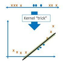
Fig. Applying kernel function for easier separation
Neural Networks
Developed in the 1950’s, neural networks are the poster child for machine learning, particularly “deep learning.”They form the basis for complex applications such as speech-to-text, image classification and object detection. If you jump right to the more sophisticated forms used for deep learning, it’s easy to be overwhelmed; but the basic functioning of a neural network is not difficult to follow.
A neural network is simply a set of mathematical transformations applied to input data as it feeds through a network of interconnected nodes (called neurons) organized in layers. Each input is represented by an input node. These nodes are connected to nodes in the next layer, with a weight assigned to each connection, loosely representing a general significance of that input. As values travel from node to node, they are multiplied by the weights for the connections and an activation function is applied. The resulting value for each node is then passed through the network to nodes in the next layer. Ultimately, an activation function in an output node assigns a value to provide the prediction.

Training a neural network is all about finding the right values for the weights. A first pass of data through the network with initial settings for weights yields output values that do not closely match the known output values from the training data. A back-propagation process uses gradient information (quantifying how a change in weight values affects outputs at each node) to adjust the weights and cycles through the network repeatedly until the weights converge to values with acceptable error between predicted and actual values.
Because of the ultra-flexibility in the combination of the number of hidden layers, the number of neurons in each layer, and the activation functions used, neural networks can provide extremely accurate predictions for highly non-linear systems. One of my favorite tools for illustrating neural networks is this cool interactive example developed by researchers from Google. Check it out…you won’t be disappointed.
With this simple explanation of neural networks serving as a foundation, you can now delve into the more advanced variants such as convolutional neural networks, recurrent neural networks, and denoising autoencoders.
The Magic is Gone
There you have it – the ideas behind four of the most popular machine learning algorithms. While these algorithms build highly predictive models, they’re not magic. A grounding in the fundamental concepts will help you understand these algorithms–and those extending them in novel ways.
Bio: Brett Wujek is a Senior Data Scientist with the R&D team in the SAS Advanced Analytics division. He helps evangelize and guide the direction of advanced analytics development at SAS, particularly in the areas of machine learning and data mining. Prior to joining SAS, Brett led the development of process integration and design exploration technologies at Dassault Systemes, helping to architect and implement industry-leading computer-aided optimization software for product design applications. His formal background is in design optimization methodologies, receiving his PhD from the University of Notre Dame for his work developing efficient algorithms for multidisciplinary design optimization.
Related:
- Fundamental Breakthrough in 2 Decade Old Algorithm Redefines Big Data Benchmarks
- Data Science Primer: Basic Concepts for Beginners
- Must-Know: What is the idea behind ensemble learning?`