 Understanding Deep Convolutional Neural Networks with a practical use-case in Tensorflow and Keras
 Understanding Deep Convolutional Neural Networks with a practical use-case in Tensorflow and Keras
We show how to build a deep neural network that classifies images to many categories with an accuracy of a 90%. This was a very hard problem before the rise of deep networks and especially Convolutional Neural Networks.
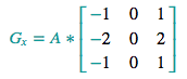
kernel = np.array([[-1, 0, 1], [-2, 0, 2], [-1, 0, 1]], np.float32)
dx = show_differences(kernel)
The white areas are the ones that better respond to the filter, indicating the presence of a vertical edge. Look closely at the cat's left ear for example and notice how its edge is captured.
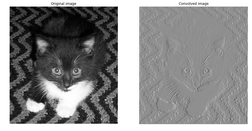
Cool, right? Here is a second filter that does the same operation but for the horizontal changes.

kernel = np.array([[1, 2, 1], [0, 0, 0], [-1, -2, -1]], np.float32)
dy = show_differences(kernel)
Notice how the whiskers are detected.
The two previous filters are gradient operators. They allow, to some extent, to reveal an inherent structure in the image with respect to a direction.
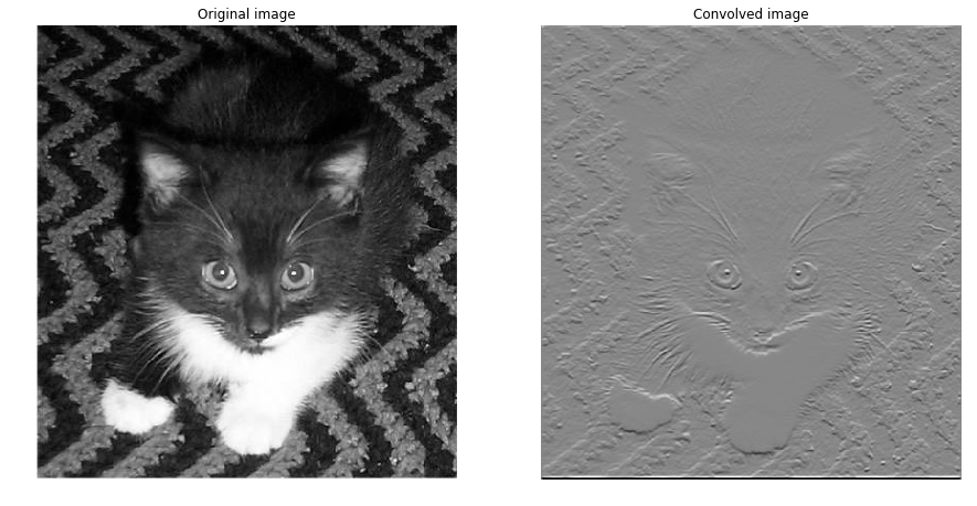
However, when G_x and G_y are combined in the following formula:
![]()
they allow an even better edge detection.
mag = np.hypot(dx, dy)  # magnitude
mag *= 255.0 / np.max(mag)  # normalize (Q&D)

fig = plt.figure(figsize=(15, 15))
plt.subplot(121)
plt.title('Original image')
plt.axis('off')
plt.imshow(image, cmap='gray')

plt.subplot(122)
plt.title('Convoluted image with highlighted edges')
plt.axis('off')
plt.imshow(mag, cmap='gray')
This is called a Sobol filter. It's a non-linear combination of two simple convolutions. We'll see later that convolution layers are capable of aggregating multiple feature maps in a non-linear fashion and therefore allowing results such that this edge detection.
There are more advanced and exotic filters out there. For additional information you can refer to this wikipedia link .
We now understand what a convolution layer does in a convnet: it generates a convolved output that responds to a visual element existing in the input. The output may be of reduced size, and you can think of it as a condensed version of the input regarding a specific feature.
The kernel determines which feature the convolution is looking for. It plays the role of the feature detector. We can think of many filters that could detect edges, semi circles, corners, etc.
More than one filter on a convolution layer?
In a typical CNN architecture, we won't have one single filter per convolution layer. Sometimes we'll have 10, 16 or 32. Sometimes more. In this case we'll be performing as many convolutions per layer as the number of filters. The idea is to generate different feature maps, each locating a specific simple characteristic in the image. The more filters we have, the more intrinsic details we extract.
Keep in mind that these simple characteritics we extract are later combined in the network to detect more complex patterns.
What about filter weights? How to choose them?
We won't handcraft filter weights based on a domain knowledge we may have about the dataset.
In practice, when training CNNs we won't be setting the filter weights manually. These values are learnt by the network. Automatically. Do you recall how weights are learnt in a typical fully connected network via backpropagation? Well, convnets do the same thing.
Instead of large weight matrices per layer, CNNs learn filter weights. In other words, this means that the network, when adjusting its weights (from random values) to decrease the classification errors, comes up with the right filters that are suitable for characterising the object we're interested in. This is a powerful idea that reverse-engineers the vision process.
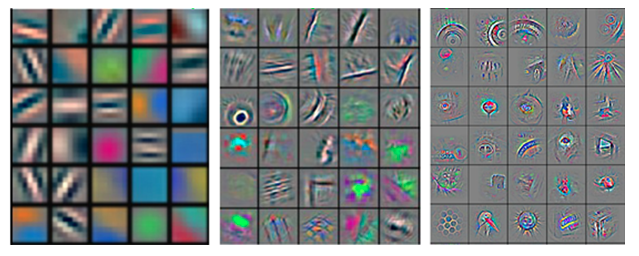
I find convnets both impressive and mysterious. Here's an example of the first three features map being learnt in a convnet. (A famous one, called AlexNet)
Note how complex the features get from simple edges to more bizarre shapes.
Weight sharing?
A feature map is produced by one and only one filter, i.e. all the hidden neurons "share" the same weights because the same filter is producing them all. That's what we call weight sharing. It's a property that makes CNNs faster to train by drastically reducing the number of learnt parameters.
In addition to speeding up training, the concept of weight sharing is motivated by the fact that a visual pattern can appear in different regions of an image many times and thus having a single filter that detect it over the whole image makes sense.
ReLu Layer
Once the feature maps are extracted from the convolution layer, the next step is to move them to a ReLU layer. ReLU layers are usually coupled with conv layers. They usually work together.
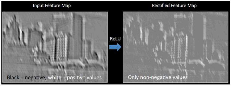
A ReLU layer applies an elemetwise ReLU function on the feature map. This basically sets all negative pixels to 0. The output of this operation is called a rectified feature map.

ReLU layers have two main advantages:
- They introduce a non-linearity in the network. In fact, all operations seen so far: convolutions, elementwise matrix multiplication and summation are linear. If we don't have a non linearity, we will end up with a linear model that will fail in the classification task.
- They speed up the training process by preventing the vanishing gradient problem.
Here's a visualization of what the ReLU layer does on an image example:
Pooling layer
The rectified feature maps now go throught a pooling layer. Pooling is a down-sampling operation that reduces the dimensionality of the feature map.
The most common pooling operation is max-pooling. It involves a small window of usally size 2x2 which slides by a stride of 2 over the rectified feature map and takes the largest element at each step.
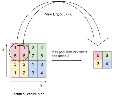
For example a 10x10 rectified feature map is converted to a 5x5 output.
Max-pooling has many benefits:
- It reduces the size of the rectified feature maps and the number of trainable parameters, thus controlling overfitting
- It condenses the feature maps by retaining the most important features
- It makes the network invariant to small transformations, distortions and translations in the input image (a small distortion in input will not change the output of Pooling – since we take the maximum value in a local neighborhood)
The intuition behind max-pooling is not straightforward. From my understanding, I schematize this as follow:
If a feature (an edge for instance) is detected, say on small portion of an image like the 2x2 red square above, we don't care what exact pixels made it appear. Instead, we pick from this portion the one with the largest value and assume that it's this pixel that summarizes the visual feature. This approach seems aggressive since it loses the spatial information. But the fact is, it's really efficient and works very well in practice. In fact you shouldn't have in mind a 4x4 image example like this. When max-pooling is applied to a relatively high resolution image, the main spatial information still remains. Only uninportant details vanish. This is why max pooling prevents overfitting. It makes the network concentrate on the most relevant information of the image.
Fully Connected Layer
CNNs also have a fully connected layer. You the one we are used to see in typical FC nets. It usually comes at the end of the network where the last pooled layer is flattened into a vector that is then fully connected to the output layer which is the prediction vector (its size is the number of classes).
If you still have the whole picture in mind (Input -> Convolution -> ReLU -> Max pooling) now add up a fully connected layer to the output and you'll have a complete and tiny convnet that assembles the basic blocks.
This may look like this:
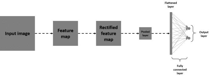
Note that the flattened layer is just a vectorized version of the pooled layer just before it.
Why do we need a fully connected layer?
Fully connected layer(s) play the role of the classification task, whereas the previous layers act as the feature extractors.
Fully connected layers take the condensed and localized results of convolutions, recitification and pooling and integrate them, combine them and perform the classification.
Apart from classification, adding a fully-connected layer is also a way of learning non-linear combinations of these features. Most of the features from convolution and pooling layers may be good for the classification task, but combinations of those features might be even better.
Think of the FC layer as an additional level of abstraction that adds up to the network.
Wrap up
Let's recap the layers what we've seen so far:
| Layer | Function |
|---|---|
| Input layer | Takes an image as input and preserves its spatial structure |
| Convolution layer | Extracts feature maps from the input, each responding to a specific pattern |
| ReLU layer | Introduces non-linearities in the network by setting negative pixels to 0 |
| Max-pooling layer | Down-samples the rectified feature maps, thus reducing the spatial dimensionality and retaining important features. This prevents overfitting |
| Fully-Connected layer | Learns non-linear combinations of the features and performs the classification task |
In a typical CNN architecture, there won't be one layer of each type.
In fact, if you consider the example of a network that has two sucessive convolutional-pooling layers, the idea is that the second convolution takes a condensed version of the image which indicates a presence or not of a particular feature. So you can think of the second conv layer as having as input a version of the original input image. That version is abstracted and condensed, but still has a lot of spatial structure.
We usually have 2 or 3 FC layers too. This allows to learn many non-linear combinations of features before proceeding to the classification task.
Let me quote Andrej Karpathy on this point:
The most common form of a ConvNet architecture stacks a few CONV-RELU layers, follows them with POOL layers, and repeats this pattern until the image has been merged spatially to a small size. At some point, it is common to transition to fully-connected layers. The last fully-connected layer holds the output, such as the class scores. In other words, the most common ConvNet architecture follows the pattern:
INPUT -> [[CONV -> RELU]N -> POOL?]M -> [FC -> RELU]*K -> FC
Now that we know the basic blocks of a convnet, let's look at a typical network.
LeNet5
Below is a popular convnet, designed by LeCun et al. in 1998. It's called LeNet5.
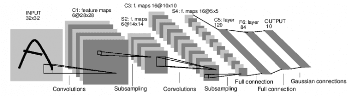
Let's tell this network architecture. I encourage you to first do this exercice by yourself.
- Input layer: a 32x32 grayscale image (1 color channel)
- Convolution layer n°1: it applies 6 different 5x5 filters on the image. This results in 6 feature maps of size 28x28 (the activation function in applied in this layer on the 6 feature maps, it was not ReLU back then)
- Pooling layer on the 6 28x28 feature maps resulting in 6 14x14 pooled feature maps (1/4 the size)
- Convolution layer n°2: it applies 16 different 5x5 filters on the 6 14x14 previous feature maps. This generates 16 feature maps of size 10x10. Each of these 16 feature maps is the sum of the six matrices that are the results of convolution between the first filter and the six inputs
- Pooling layer on the 16 10x10 feature map resulting in 16 5x5 pooled maps
- A first fully connected layer containing 120 neurons. Each neurons is connected to all the pixels of the 16 5x5 feature maps. This layer has 16x5x5x120=48000 learnable weights
- A second fully connected layer containing 84 neurons. This layer is fully connected to the previous one. It has 120x84=10080 learnable weights.
- A fully connected layer to the output layer. 84x10=840 learnable weights.
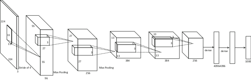
More advanced CNN architectures
If you're interested in more complex and state of the art convnets architectures, you can read about them in this blog.
Below a popular CNN that won the 2012 ImageNet competition (AlexNet).
3 - Setting Up a Deep Learning Evironment
Deep learning is computationally very heavy. You'll figure this out when you'll prototype your first model on your laptop.
However, the training can be drastically sped up when you use Graphics Processing Units (GPUs). The reason is that GPUs are very efficient at paralellizing tasks such as matrix mutliplications. And since neural nets are all about matrix multiplications, the performence in incredibly boosted.
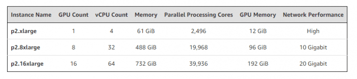
I don't have a powerful GPU on my laptop. So I used a virtual machine on Amazon Web Services (AWS). It's called p2.xlarge and is part of Amazon EC2 instances. It has an Nvidia GPU with 12GB of video memory, 61GB of RAM, 4vCPU and 2,496 CUDA cores. It's a powerful beast and it costs $0.9 per hour.
There are of course more powerful instances but for the given task we're tackling, a p2.xlarge is more than enough.
I started this instance on the Deep Learning AMI CUDA 8 Ubuntu Version. Here to know more about it.
It's basically a setting of an Ubuntu 16.04 server that encapsulates all the deep learning frameworks needed (Tensorflow, Theano, Caffe, Keras) as well as the GPU drivers (which I heard are a nightmare to install...)
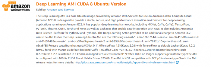
This is great: AWS provides with you with powerful instances and ready-to-use Deep learning dedicated environments so that you can start working on your projects really fast.
If you're not familiar with AWS you can look at these two posts:
- https://blog.keras.io/running-jupyter-notebooks-on-gpu-on-aws-a-starter-guide.html
- https://hackernoon.com/keras-with-gpu-on-amazon-ec2-a-step-by-step-instruction-4f90364e49ac
They should get you started to:
- Set up an EC2 VM and connect to it
- Configure the network security to access jupyter notebook remotely
4 - Building a cat/dog classifier using Tensorfow and Keras
The environment is now set up. We're ready to put in practice what we've learnt so far and build a convnet that classifies images of cats and dogs.
We're going to use the Tensorflow deep learning framework and Keras.
Keras is a high-level neural networks API, written in Python and capable of running on top of TensorFlow, CNTK, or Theano. It was developed with a focus on enabling fast experimentation. Being able to go from idea to result with the least possible delay is key to doing good research.

4 - 1 Builiding a convnet from scratch
In this first section, we'll setup an end-to-end pipeline to train a CNN. We'll go through data preparation and augmentation, architecture design, training and validation. We'll plot the loss and accuracy metrics on both the train and validation set: this will allow us to assess the improvement of the model over the training.
Data preparation
The first thing to do before starting is to download and unzip the train dataset from Kaggle.
%matplotlib inline
from matplotlib import pyplot as plt
from PIL import Image
import numpy as np
import os
import cv2
from tqdm import tqdm_notebook
from random import shuffle
import shutil
import pandas as pd
We must now organize the data so that it's easily processed by keras.
We'll create a data folder in which we'll have in two subfolders:
- train
- validation
Each of them will have 2 folders:
- cats
- dogs
At the end we'll have the following structure:
data/
    train/
        dogs/
            dog001.jpg
            dog002.jpg
            ...
        cats/
            cat001.jpg
            cat002.jpg
            ...
    validation/
        dogs/
            dog001.jpg
            dog002.jpg
            ...
        cats/
            cat001.jpg
            cat002.jpg
This structure will allow our model to know from which folder to fetch the images as well as their labels for either training or validation.
Here's a function that allows you to construct this file tree. It has two parameters: the total number of images nand the ratio of validation set r.
def organize_datasets(path_to_data, n=4000, ratio=0.2):
    files = os.listdir(path_to_data)
    files = [os.path.join(path_to_data, f) for f in files]
    shuffle(files)
    files = files[:n]

    n = int(len(files) * ratio)
    val, train = files[:n], files[n:]


    shutil.rmtree('./data/')
    print('/data/ removed')

    for c in ['dogs', 'cats']:
        os.makedirs('./data/train/{0}/'.format(c))
        os.makedirs('./data/validation/{0}/'.format(c))

    print('folders created !')

    for t in tqdm_notebook(train):
        if 'cat' in t:
            shutil.copy2(t, os.path.join('.', 'data', 'train', 'cats'))
        else:
            shutil.copy2(t, os.path.join('.', 'data', 'train', 'dogs'))

    for v in tqdm_notebook(val):
        if 'cat' in v:
            shutil.copy2(v, os.path.join('.', 'data', 'validation', 'cats'))
        else:
            shutil.copy2(v, os.path.join('.', 'data', 'validation', 'dogs'))

    print('Data copied!')
I used:
- n : 25000 (the entire dataset)
- r : 0.2
ratio = 0.2
n = 25000
organize_datasets(path_to_data='./train/', n=n, ratio=ratio)
Let's load Keras and its dependencies.
import keras
from keras.preprocessing.image import ImageDataGenerator
from keras_tqdm import TQDMNotebookCallback
from keras.models import Sequential
from keras.layers import Dense
from keras.layers import Dropout
from keras.layers import Flatten
from keras.constraints import maxnorm
from keras.optimizers import SGD
from keras.layers.convolutional import Conv2D
from keras.layers.convolutional import MaxPooling2D
from keras.utils import np_utils
from keras.callbacks import Callback
Image generators and data augmentation
When training a model, we're not going to load the entire dataset in memory. This won't be efficient, especially if you use your local machine.
We're going to use the ImageDataGenerator class. It allows you to indefinitely stream the images by batches from the train and validation folders. Every batch flows through the network, makes a forward-prop, a back-prop then a parameter updates (along with the test on the validation data). Then comes the next batch and does the same thing, etc.
Inside the ImageDataGenerator object, we're going to introduce random modifications on each batch. It's a process we call data augmentation. It allows to generate more data so that our model would never see twice the exact same picture. This helps prevent overfitting and makes the model generalize better.
We'll create two ImageDataGenerator objects.
train_datagen for the training set and val_datagen one for the validation set. The two of them will apply a rescaling on the image, but the train_datagen will introduce more modifications.
batch_size = 32

train_datagen = ImageDataGenerator(rescale=1/255.,
                                    shear_range=0.2,
                                    zoom_range=0.2,
                                    horizontal_flip=True
                                    )
val_datagen = ImageDataGenerator(rescale=1/255.)
From the two previous objects we're going to create two file generators:
- train_generator
- validation_generator
Each one generates, from its directory, batches of tensor image data with real-time data augmentation. The data will be looped over (in batches) indefinitely.
train_generator = train_datagen.flow_from_directory(
        './data/train/',
        target_size=(150, 150),
        batch_size=batch_size,
        class_mode='categorical')

validation_generator = val_datagen.flow_from_directory(
        './data/validation/',
        target_size=(150, 150),
        batch_size=batch_size,
        class_mode='categorical')

##Found 20000 images belonging to 2 classes.
##Found 5000 images belonging to 2 classes.
Model architecture
I'll use a CNN with three convolution/pooling layers and two fully connected layers.
The three conv layers will use respectively 32, 32 and 64 3x3 filters.
I used dropout on the two fully connected layers to prevent overfitting.
model = Sequential()

model.add(Conv2D(32, (3, 3), input_shape=(150, 150, 3), padding='same', activation='relu'))
model.add(MaxPooling2D(pool_size=(2, 2)))

model.add(Conv2D(32, (3, 3), padding='same', activation='relu'))
model.add(MaxPooling2D(pool_size=(2, 2)))

model.add(Conv2D(64, (3, 3), activation='relu', padding='same'))
model.add(MaxPooling2D(pool_size=(2, 2)))

model.add(Dropout(0.25))
model.add(Flatten())
model.add(Dense(64, activation='relu'))
model.add(Dropout(0.5))
model.add(Dense(2, activation='softmax'))
I used the stochastic gradient descent optimizer with a learning rate of 0.01 and a momentum of 0.9.
Since we're having a binary classification, I used the binary crossentropy loss function.
epochs = 50
lrate = 0.01
decay = lrate/epochs
sgd = SGD(lr=lrate, momentum=0.9, decay=decay, nesterov=False)
model.compile(loss='binary_crossentropy', optimizer=sgd, metrics=['accuracy'])
Keras provides a convenient method to display a summary of the model. For each layer, this shows up the output shape and the number of trainable parameters.
This a sanity check before starting fitting the model.
model.summary()

Let's look at the network architecture:
Visualizing the architecture

Training the model
Before training the model, I defined two callback functions that will be called while training.
- One for early stopping the training when the loss function stops improving on the validation data
- One for storing the validation loss and accuracy of each epoch: this allows to plot the training error
## Callback for loss logging per epoch
class LossHistory(Callback):
    def on_train_begin(self, logs={}):
        self.losses = []
        self.val_losses = []

    def on_epoch_end(self, batch, logs={}):
        self.losses.append(logs.get('loss'))
        self.val_losses.append(logs.get('val_loss'))

history = LossHistory()

## Callback for early stopping the training
early_stopping = keras.callbacks.EarlyStopping(monitor='val_loss',
                              min_delta=0,
                              patience=2,
                              verbose=0, mode='auto')
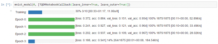
I also used keras-tqdm which is an awesome progress-bar that perfectly integrates with Keras.
It allows you to monitor the training of you models very easily.
What you need to do is simply load the TQDMNotebookCallback class from keras_tqdm then pass it as a third callback functions.
Here's what keras-tqdm looks like on simple example:
A few words about the training:
- We'll use the fit_generator method which is a variant (of the standard fit method) that takes a generator as input.
- We'll train the model over 50 epochs: over one epoch 20000 unique and augmented images will flow by batch of 32 to the network, performing a forward and back propagation and adjusting the weights with SGD. The idea of using multiple epochs is to prevent overfitting.
fitted_model = model.fit_generator(
        train_generator,
        steps_per_epoch= int(n * (1-ratio)) // batch_size,
        epochs=50,
        validation_data=validation_generator,
        validation_steps= int(n * ratio) // batch_size,
        callbacks=[TQDMNotebookCallback(leave_inner=True, leave_outer=True), early_stopping, history],
        verbose=0)
This is a heavy computation:
- If you're on your laptop this may take about 15 minutes per epoch
- If you're using an the p2.xlarge EC2 instance like me, this takes about 2 minutes or so per epoch
tqdm allows you to monitor the validation loss and accuracy on each epochs. This is useful to check the quality of your model.
Classification results
We reached 89.4% accuracy (on the validation data) in 34 epochs (training/validation error and accuracy displayed below)
This is a good result given that I didn't invest too much time designing the architecture of the network.
Now let's save the model for later use.
model.save('./models/model4.h5')
Let's plot the train and validation losses on the same graph:
losses, val_losses = history.losses, history.val_losses
fig = plt.figure(figsize=(15, 5))
plt.plot(fitted_model.history['loss'], 'g', label="train losses")
plt.plot(fitted_model.history['val_loss'], 'r', label="val losses")
plt.grid(True)
plt.title('Training loss vs. Validation loss')
plt.xlabel('Epochs')
plt.ylabel('Loss')
plt.legend()
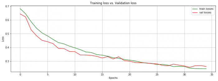
We interrupt the training when the validation loss doesn't improve on two successive epochs.
Let's now plot the accuracy on both the training set and validation set.
losses, val_losses = history.losses, history.val_losses
fig = plt.figure(figsize=(15, 5))
plt.plot(fitted_model.history['acc'], 'g', label="accuracy on train set")
plt.plot(fitted_model.history['val_acc'], 'r', label="accuracy on validation set")
plt.grid(True)
plt.title('Training Accuracy vs. Validation Accuracy')
plt.xlabel('Epochs')
plt.ylabel('Loss')
plt.legend()
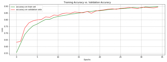
These two metrics keep increasing before reaching a plateau where the model eventually starts overfitting (from epoch 34).
4 - 2 Loading a pre-trained model
So far so good: we designed a custom convnet that performs reasonably well on the valiation data with ~ 89% accuracy.
There is however a way to get a better score: loading the weights of a pre-trained convnet on a large dataset that includes images of cats and dogs among 1000 classes. Such a network would have learnt relevant features that are relevant to our classification.
I'll load the weights of the VGG16 network: more specifically, I'm going to load the network weights up to the last conv layer. This network part acts as a feature detector to which we're going to add fully connected layers for our classification task.
VGG16 is a very large network in comparison to LeNet5. It has 16 layers with trainable weights and around 140 millions parameters. To learn more about VGG16 please refer to this pdf link.
We first start by loading the VGG16 weights (trained on ImageNet) by specifying that we're not interested in the last three FC layers.
from keras import applications
# include_top: whether to include the 3 fully-connected layers at the top of the network.
model = applications.VGG16(include_top=False, weights='imagenet')
datagen = ImageDataGenerator(rescale=1. / 255)
Now we pass the images through the network to get a feature representation that we'll input to a neural network classifier.
We do this for the training set and the validation set.
generator = datagen.flow_from_directory('./data/train/',
                                        target_size=(150, 150),
                                        batch_size=batch_size,
                                        class_mode=None,
                                        shuffle=False)

bottleneck_features_train = model.predict_generator(generator, int(n * (1 - ratio)) // batch_size)
np.save(open('./features/bottleneck_features_train.npy', 'wb'), bottleneck_features_train)

##Found 20000 images belonging to 2 classes.

generator = datagen.flow_from_directory('./data/validation/',
                                        target_size=(150, 150),
                                        batch_size=batch_size,
                                        class_mode=None,
                                        shuffle=False)

bottleneck_features_validation = model.predict_generator(generator, int(n * ratio) // batch_size,)
np.save('./features/bottleneck_features_validation.npy', bottleneck_features_validation)

##Found 5000 images belonging to 2 classes.
When the images are passed to the network, they are in the right orders. So we associate the labels to them easily.
train_data = np.load('./features/bottleneck_features_train.npy')
train_labels = np.array([0] * (int((1-ratio) * n) // 2) + [1] * (int((1 - ratio) * n) // 2))

validation_data = np.load('./features/bottleneck_features_validation.npy')
validation_labels = np.array([0] * (int(ratio * n) // 2) + [1] * (int(ratio * n) // 2))
Now we design a small fully connected network that plugs in to the features extracted from the VGG16 and acts as the classification part of a CNN.
model = Sequential()
model.add(Flatten(input_shape=train_data.shape[1:]))
model.add(Dense(512, activation='relu'))
model.add(Dropout(0.5))
model.add(Dense(256, activation='relu'))
model.add(Dropout(0.2))
model.add(Dense(1, activation='sigmoid'))

model.compile(optimizer='rmsprop',
              loss='binary_crossentropy', metrics=['accuracy'])

fitted_model = model.fit(train_data, train_labels,
          epochs=15,
          batch_size=batch_size,
          validation_data=(validation_data, validation_labels[:validation_data.shape[0]]),
          verbose=0,
          callbacks=[TQDMNotebookCallback(leave_inner=True, leave_outer=False), history])
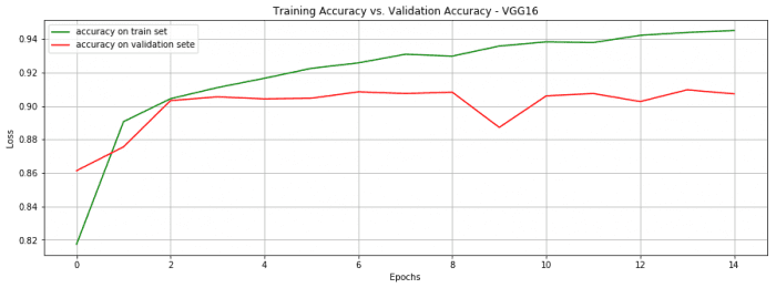
We reached 90.7% accuracy on 15 epochs only. Quite not bad. Note that each epoch takes around 1 minute on my personal laptop.
fig = plt.figure(figsize=(15, 5))
plt.plot(fitted_model.history['loss'], 'g', label="train losses")
plt.plot(fitted_model.history['val_loss'], 'r', label="val losses")
plt.grid(True)
plt.title('Training loss vs. Validation loss - VGG16')
plt.xlabel('Epochs')
plt.ylabel('Loss')
plt.legend()
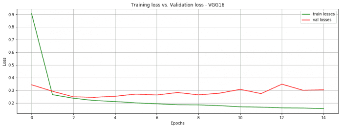
fig = plt.figure(figsize=(15, 5))
plt.plot(fitted_model.history['acc'], 'g', label="accuracy on train set")
plt.plot(fitted_model.history['val_acc'], 'r', label="accuracy on validation sete")
plt.grid(True)
plt.title('Training Accuracy vs. Validation Accuracy - VGG16')
plt.xlabel('Epochs')
plt.ylabel('Loss')
plt.legend()
Many deep learning pioneers encourage to use pre-trained networks for classification tasks. In fact, this usually leverages the training of a very large network on a very large dataset.
Keras allows you easliy to download pretrained networks like VGG16, GoogleNet and ResNet. More about this here.
The general motto is:
Don't be a hero. Don't reinvent the wheel. Use pre-trained networks!
Where to go from here ?
If you're interested in improving a custom CNN:
- On the dataset level, introduce more data augmentation
- Play with the network hyperparameters: number of conv layers, number of filters, size of the filters. Have a validation dataset to test each combination.
- Change the optimizer or tweak it
- Try different cost functions
- Use more FC layers
- Introduce more aggressive dropout
If you're interested in having better results with pretrained networks:
- Use different network architectures
- Use more FC layers with more hidden units
If you want to do discover what the CNN model has learnt:
- Visualize feature maps. I haven't done that yet, but there's an interesting paper on the subject
If you want to use the trained model:
- Ship it in a web app and use it on new cat/dog images. This is a good exercise to see if the model generalizes well.
Conclusion
This article was an opportunity to go through the theory behind convolutional neural networks and explain each of their principal components in more details.
This was also a hands-on guide to setup a deep learning dedicated environment on AWS and develop an end-to-end model from scratch as well as an enhanced model based on a pre-trained one.
Using python for deep learning is extermely fun. Keras made it easier for preprocessing the data and building up the layers. Keep in mind that if you want someday to build custom neural net components, you'll have to switch to another framework.
I hope this gave you a practical intuition about the convnets mechanisms and a strong appetite to learn more.
Convnets are amazingly powerful. Anyone working on computer vision believes in their robustness and efficiency.
Their applications are getting a larger scope. NLP practictioners are now the ones who are switching to convnets. Here are some of their applications:
- Text classification using CNNs : link
- Automated image captioning (Image + Text): link
- Text classification at character level: link
References
Here's a list of some references I used to learn about neural nets and convnets:
- neuralnetworksanddeeplearning.com : By far the best notes on neural networks and deep learning. I highly recommend this website to anyone who want to start learning about neural nets.
- CS231n Convolutional Neural Networks for Visual Recognition : Andrej Karpathy's lectures at Stanford. Great mathematical focus.
- A Beginner Guide to Understanding Neural Networks: A three-part post explaining CNNs, from the basic high level inuition to the architecture details. Very interesting read. Learnt a lot from it.
- Running jupyter notebooks on GPU on AWS
- Building powerful image classification models using very little data
- CatdogNet - Keras Convnet Starter
- A quick introduction to Neural Networks
- An Intuitive Explanation of Convolutional Neural Networks
- Visualizing parts of Convolutional Neural Networks using Keras and Cats
Bio: Ahmed Bebes Graduated from Telecom Paristech and HEC Paris. He is a tech enthusiast, machine learning practitioner and open-source aficionado. Interested in big data and disruptive web technologies.
Original. Reposted with permission.
Related