 Understanding Deep Convolutional Neural Networks with a practical use-case in Tensorflow and Keras
 Understanding Deep Convolutional Neural Networks with a practical use-case in Tensorflow and Keras
We show how to build a deep neural network that classifies images to many categories with an accuracy of a 90%. This was a very hard problem before the rise of deep networks and especially Convolutional Neural Networks.
By Ahmed Besbes
Original. Reposted with permission.
Deep learning is one of the most exciting artificial intelligence topics. It's a family of algorithms loosely based on a biological interpretation that have proven astonishing results in many areas: computer vision, natural language processing, speech recognition and more.
Over the past five years, deep learning expanded to a broad range of industries.
Many recent technological breakthroughs owe their existence to it. To name a few: Tesla autonomous cars, photo tagging systems at Facebook, virtual assistants such as Siri or Cortana, chatbots, object recognition cameras. In so many areas, deep learning achieved a human-performance level on the cognitive tasks of language understanding and image analysis.
Here's an example of what deep learning algorithms are capable of doing: automatically detecting and labeling different objects in a scene.

Deep learning also became a widely covered tech topic.

In this article, I'll go beyond the overall hype you'd encounter in the mass media and present a concrete application of deep learning.
I'll show you how to build a deep neural network that classifies images to their categories with an accuracy of a 90%. This seemingly simple task is a very hard problem that computer scientists have been working on for years before the rose of deep networks and especially Convolutional Neural Networks (CNN).
This post is broken into 4 parts where I will:
- Present the dataset and the use-case and explain the complexity of the image classification task
- Go over the details about Convolutional Neural Nets. I'll explain their inner meachanisms and the reason why they are more suitable to image classification than ordinary neural netwoks
- Set up a deep learning dedicated environment on a powerful GPU-based EC2 instance from Amazon Web Services (AWS)
- Train two deep learning models: one from scratch in an end-to-end pipeline using Keras and Tensorflow, and another one by using a pre-trained network on a large dataset
These parts are independent. If you're not interested in the theory you can skip part 1 and 2.
Deep learning is a challenging topic to handle. As a machine learning practitioner, I myself spent a lot of time learning about the subject. In the last part, I'll share all the material I used so that you can use it yourself and start your deep learning journey.
This article is an honest attempt to synthesize the knowledge I've developed on neural nets. So please don't hesitate to point out any mistake you come across while reading. Feel free to also discuss any point you see unclear or any thought you'd like to share.
In case you're willing to reproduce my work or send a pull request, the code of this article as well as the trained models are available in my github account
Let's get started.
1 - A fun use case: How to classify cats and dogs?
There are lots of image datasets dedicated to benchmarking deep learning models.
The one I'll be using in this article comes from the Cat vs Dogs Kaggle competition . As you've probably guessed it, it's a set of labeled images of cats and dogs.
Like in every Kaggle competition, we'll have tow folders:
- A train folder: it contains 25,000 images of dogs and cats. Each image in this folder has the label as part of the filename. We'll use it to train and validate our model.
- A test folder: it contains 12,500 images, named according to a numeric id. For each image in this dataset, one should predict a probability that the image is a dog (1 = dog, 0 = cat). In practice it's used to score the model on the Kaggle leaderboard.
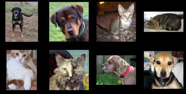
As you can see, we have a variety of images. They all are in different resolutions. Cats and dogs are in different shapes, positions, colors. They may be sitting, they may not. They may be happy or sad. Cats may be sleeping, dogs may be barking. Photographs can be taken from different angles with a different zoom.
An infinite number of configurations is possible. For a human, recognizing pets in a scene in a set of heterogeneous photographs comes naturally with no effort. This is however not a trivial task for a machine. In fact, automatic classification assumes to know how to robustly describe what makes a cat a cat and makes a dog a dog. This assumes to know the intrinsic features that describe each animal.
What makes deep neural networks very effective at classifying images is their ability to automatically learn multiple levels of abstraction that simply characterize each class in a given classification task. They can recognize patterns with extreme variability, and with robustness to distortions and simple geometric transformations.
Let's see how deep neural nets handle this.
2 - Fully Connected Networks vs CNNs
Many people started using Fully Connected networks to address the image classification problem. However, they came to realize that these networks are not fully optimal for the task.
Let's understand why.
2 - 1 A Fully Connected (FC) Neural Network
Fully connected neural nets are networks where each neuron is connected to every neuron in the adjacent layers. They are the standard and typical neural network architectures. To learn more about the theory behind neural networks please refer to this link and this one: These are Andrej Karpathy's Stanford lectures and they are simply, awesome.
To illustrate, here's a 3-hidden layer FC neural net.
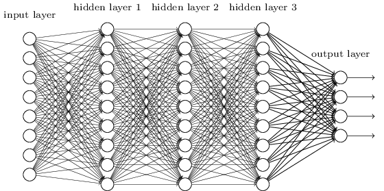
Using FC networks, images are first converted to a one dimensional vector before being fed as an input.
For example, a color image of size 256x256, which is represented by object of shape (255, 255, 3) where 3 is the number of color channels, is converted to a vector of size 256 x 256 x 3 = 196608. All we did here was rolling the image into a long vector. Each element of this vector is a pixel value.
Fully connected networks can be very good classifiers. In the realm of supervised algorithms, they can learn complex non-linear patterns and generalize well assuming we design a robust architecture that doesn't overfit on the data.
When it comes to processing images, fully connected networks are unfortunately not the right tools.
I see two main reasons:
- Let's imagine that we have one hidden layer of 1000 hidden units for our case. 1000 is a reasonable value given the size of the input layer. With this configuration, the number of parameters (or weights) connecting our input layer to the first hidden layer is equal to 196608 x 1000 = 196608000! This is not only a huge number but the network is also not likely to perform very well given that neural networks need in general more than one hidden layer to be robust. But fair enough. Let's say that our network is very good with that one hidden layer and 1000 hidden units. Let's do the math for the memory cost. A weight is a floating value that is encoded in 8 bytes. 196698000 weights would then cost ... 1572864000 bytes which is an approximate value of ~ 1,572 GB . So we'll need 1,572 GB to store the weights of the first hidden layer only. Unless you have a lot of RAM on your laptop, this is clearly not a scalable solution.
- With fully connected networks, we lose the spatial structure that is intrinsic to the image. In fact, after converting the image to a long vector, each pixel value is processed by the network pretty much the same as the other pixels. There is no assumption of spatial correlation between the pixels whatsoever. Each pixel has the same role. This is unfortunately a huge information loss since we lose the dependencies and the similarities between closer pixels. This is an infromation that we want to be encoded in our model.
To overcome these two limitations, a lot of work have been invested to come up with new neural network architectures that are both scalable and suitable to handle the complexity of the image data.
And that's when we came up with Convolutional Neural Networks (CNNs).
2 - 2 Convolutional Neural Networks
Convolutional Neural Networks (or CNNs) are special kind of neural architectures that have been specifically designed to handle image data. Since their introduction by (LeCun et al, 1989) in the early 1990's, CNNs have demonstrated excellent performance at tasks such as handwritten digit classification and face detection. In the past few years, several papers have shown that they can also deliver outstanding results on more challenging visual classification tasks. Most notably (Krizhevsky et al., 2012) show record beating performance on the ImageNet 2012 classification benchmark, with their convnet model (AlexNet) achieving an error rate of 16.4% compared to the second place result of 26.1%.
CNNs are not just hype. Several factors are responsible for the renewed interest people got in them.
- The availability of very large training datasets with millions of labeled examples. One of the most popular databases is ImageNet
- Powerful GPU implementations, making the training of very large models practical
- Enhanced model regularization strategies such as Dropout
CNN are powerful at the image classification task. They are, by design, a solution to the two previous limitations that are faced by FC networks.
CNNs have their own structure and properties. They look different (and we will see it) from standard FC networks but they share the same mechanisms. In both cases, we talk about hidden layers, weights, biases, hidden neurons, loss functions, backpropagation and stochastic gradient descent. Again, if you're not familiar with these concepts, I encourage you to look at Andrej Karpathy's lectures on Neural Nets.
CNNs are composed of five basic blocks: understanding them should give you a clear intuition about the global mechanism.
- An input layer
- Convolutional layer
- ReLU layer
- Pooling layer
- Fully Connected layer
Before diving in each block, here's full CNN architecture.
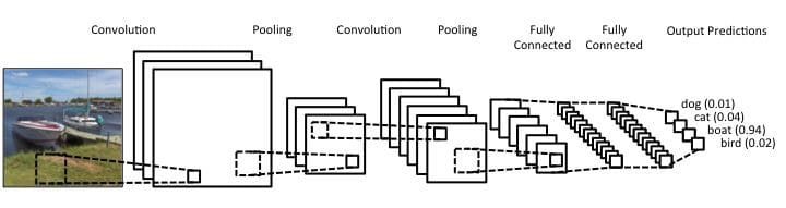
As you can see, the image is processed throughout the network over many layers and the output neurons hold the predictions for each class.
Let's understand what each layer does in details.
The input layer
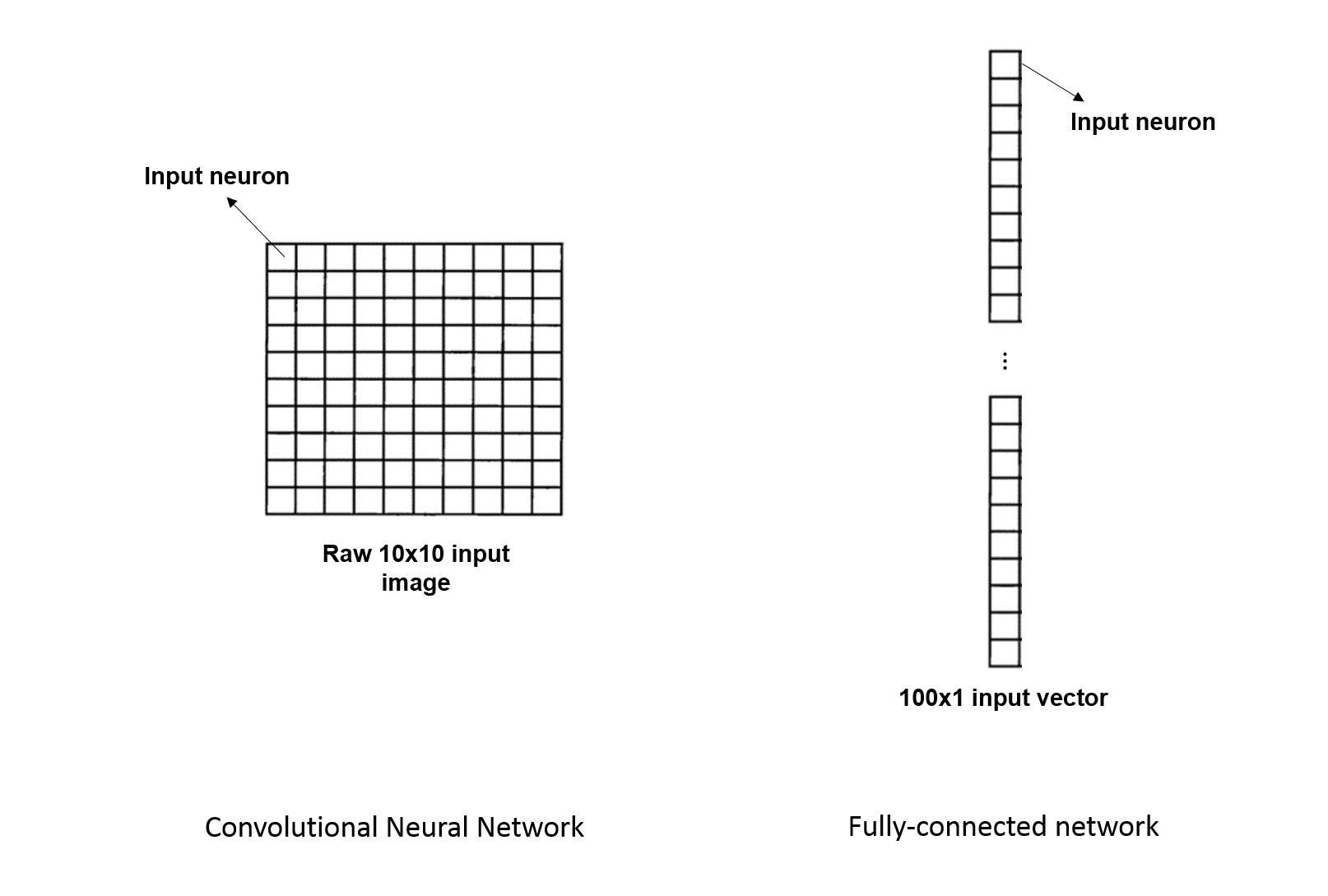
In fully connected networks, the inputs are depicted as vertical lines of neurons, basically vectors. Whether we process images or not, we always have to tweak our data to switch to this configuration.
In a convnet, however, when dealing with images, it helps to think about them as squares or neurons where each neuron represents a pixel value. Basically CNNs keep images as they are and don't try to squeeze them in a vector.
The diagram below shows the difference:
The convolution layer
This layer is the main component of a convnet. Before explaining what it does, we must first understand the main difference between convnets and FC nets in terms of connectivity. This is a crucial idea. Let me explain:
We saw it earlier: Fully Connected Networks are literally "fully connected". Or dense, if you wish. This simply means that every neuron in a given layer is connected to all the neurons of the adjacent layers. When a multi dimensional data point flows from one layer to another, the activation of each neuron in a given layer is determined by the weights of all neurons in the previous layers. These guys all have a saying.
However, things are a bit different for CNNs. They are not fully connected.
This means that each neuron in a hidden layer is not connected to all neurons of the previous layer. It is rather connected to a patch (generally a small square region) of neurons in the previous layer.
Here's an example:
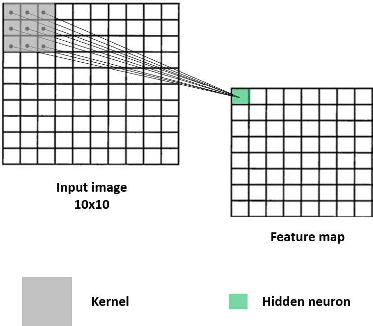
In this figure, the first neuron of the first hidden layer, which we also call a feature map, is connected to a patch of 3x3 pixels in the input. This hidden neuron depends only on this small region and will ultimately, throughout the learning, capture its characteristics.
What does the value of this first hidden neuron represent? This is the result of a convolution between a weight matrix called the kernel (the little gray square) and a small region of same size in the image, called the receptive field.
The operation behind is very simple: it's an element-wise multiplication of two matrices: the 3x3 image region and the kernel of same size. The multiplications are then summed up into an output value. In this example, we have 9 multiplications that are summed into the first hidden neuron.
This neuron basically learns a visual pattern out of the receptive field. You can think of its value as a intensity that characterises the presence or not of a feature in the image.
Now what about the other hidden neurons? How are they computed?
To compute the second hidden neuron, the kernel shifts by a unit (or one stride) on the input image from left to right and applies the same convolution, again with the same filter. Here's how it goes.
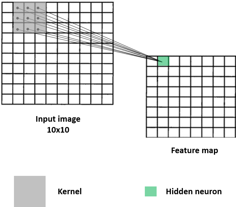
Ok now let's imagine that the kernel slides over the whole image making a convolution at each step and storing the outputs in the feature map. In practice, this is how it looks like.

This is what the convolution layer does: given a filter, it scans the input and generates a feature map.
But what does this convolution operation really represent? How to interpret the resulting feature map?
I started by stating that convolution layers capture visual patterns within an image. Let me illustrate this to convince you.
I'm going to load a cat image from the dataset. I'll then apply different convolutions on it, changing the kernel each time, and visualizing the results.
%matplotlib inline
from scipy.signal import convolve2d
import numpy as np
import cv2
from matplotlib import pyplot as plt

image = cv2.imread('./data/train/cats/cat.46.jpg')
# converting the image to grayscale
image = cv2.cvtColor(image, cv2.COLOR_BGR2GRAY)
I'll define a function that takes a kenel as an input, performs a convolution on the image and then plots the original image and the convolved one next to it.
The kernel is a small square matrix (gray square in the figures above).
def show_differences(kernel):
    convolved = convolve2d(image, kernel)
    fig = plt.figure(figsize=(15, 15))
    plt.subplot(121)
    plt.title('Original image')
    plt.axis('off')
    plt.imshow(image, cmap='gray')

    plt.subplot(122)
    plt.title('Convolved image')
    plt.axis('off')
    plt.imshow(convolved, cmap='gray')
    return convolved
Let's start by this filter:
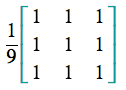
It's called box blur. When this filter is applied to a pixel value in the input image, it basically takes this pixel and its 8 neighbors (that's why we have 1 everywhere) and compute their average pixel value (that's why we devide by 9).
Mathematically, this is a simple average. Visually, it results in smoothing abrupt contrast transitions that appear in the image.
Box blur is highly used in noise removal.
Let's apply it on a cat image and see what it does.
kernel = np.array([[1, 1, 1], [1, 1, 1], [1, 1, 1]])/9
output = show_differences(kernel)

If you closely look at the convolved image, you'll notice that it's smoother, with less white pixels (noise) sprinkled on it.
Now let's look at a more aggressive blurring filter:

kernel = np.ones((8,8), np.float32)/64
dx = show_differences(kernel)

Some filters are used to capture intrinsic image details like edges.
Here is one example that computes an approximation of the vertical changes in the image A.