fast.ai Deep Learning Part 2 Complete Course Notes
This posts is a collection of a set of fantastic notes on the fast.ai deep learning part 2 MOOC freely available online, as written and shared by a student. These notes are a valuable learning resource either as a supplement to the courseware or on their own.
By Hiromi Suenaga, fast.ai Student
Editor's note: This is one of a series of posts which act as a collection of a set of fantastic notes on the fast.ai machine learning and deep learning learning streams that are freely available online. The author of all of these notes, Hiromi Suenaga -- which, in sum, are a great supplement review material for the course or a standalone resource in their own right -- wanted to ensure that sufficient credit was given to course creators Jeremy Howard and Rachel Thomas in these summaries.
Below you will find links to the posts in this particular series, along with an excerpt from each post. Find more of Hiromi's notes here.
My personal notes from machine learning class. These notes will continue to be updated and improved as I continue to review the course to “really” understand it. Much appreciation to Jeremy and Rachel who gave me this opportunity to learn.
Deep Learning 2: Part 2 Lesson 8
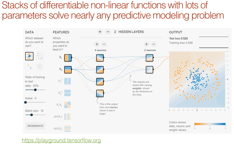
Yann LeCun has been promoting the idea that we do not call this “deep learning” but “differentiable programming”. All we did in part 1 was really about setting up a differentiable function and a loss function that describes how good the parameters are and then pressing go and it makes it work. If you can configure a loss function that scores how good something is doing your task and you have a reasonably flexible neural network architecture, you are done.
Deep Learning 2: Part 2 Lesson 9
Question: What is the intuition behind using dropout after a BatchNorm? Doesn’t BatchNorm already do a good job of regularizing [19:12]? BatchNorm does an okay job of regularizing but if you think back to part 1 when we discussed a list of things we do to avoid overfitting and adding BatchNorm is one of them as is data augmentation. But it’s perfectly possible that you’ll still be overfitting. One nice thing about dropout is that is it has a parameter to say how much to drop out. Parameters are great specifically parameters that decide how much to regularize because it lets you build a nice big over parametrized model and then decide on how much to regularize it. Jeremy tends to always put in a drop out starting with p=0 and then as he adds regularization, he can just change the dropout parameter without worrying about if he saved a model he want to be able to load it back, but if he had dropout layers in one but no in another, it will not load anymore. So this way, it stays consistent.
Deep Learning 2: Part 2 Lesson 10
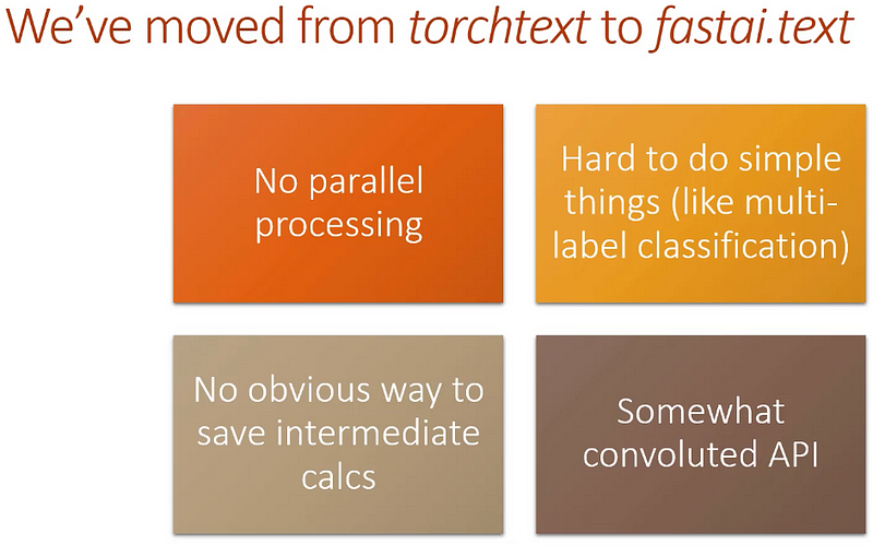
For NLP, last part, we relied on a library called torchtext but as good as it was, I’ve since then found the limitation of it too problematic to keep using it. As a lot of you complained on the forums, it’s pretty darn slow partly that’s because it’s not doing parallel processing and partly it’s because it doesn’t remember what you did last time and it does it all over again from scratch. Then it’s hard to do fairly simple things like a lot of you were trying to get into the toxic comment competition on Kaggle which was a multi-label problem and trying to do that with torchtext, I eventually got it working but it took me like a week of hacking away which is kind of ridiculous. To fix all these problems, we’ve created a new library called fastai.text. Fastai.text is a replacement for the combination of torchtext and fastai.nlp. So don’t use fastai.nlp anymore — that’s obsolete. It’s slower, it’s more confusing, it’s less good in every way, but there’s a lot of overlaps. Intentionally, a lot of the classes and functions have the same names, but this is the non-torchtext version.
Deep Learning 2: Part 2 Lesson 11
Let’s build a sequence-to-sequence model! We are going to be working on machine translation. Machine translation is something that’s been around for a long time, but we are going to look at an approach called neural translation which uses neural networks for translation. Neural machine translation appeared a couple years ago and it was not as good as the statistical machine translation approaches that use classic feature engineering and standard NLP approaches like stemming, fiddling around with word frequencies, n-grams, etc. By a year later, it was better than everything else. It is based on a metric called BLEU — we are not going to discuss the metric because it is not a very good metric and it is not interesting, but everybody uses it.
Deep Learning 2: Part 2 Lesson 12
Question: In ResNet, why is bias usually set to False in conv_layer? Immediately after the Conv, there is a BatchNorm. Remember, BatchNorm has 2 learnable parameters for each activation — the thing you multiply by and the thing you add. If we had bias in Conv and then add another thing in BatchNorm, we would be adding two things which is totally pointless — that’s two weights where one would do. So if you have a BatchNorm after a Conv, you can either tell BatchNorm not to include the add bit or easier is to tell Conv not to include the bias. There is no particular harm, but again, it’s going to take more memory because that is more gradients that it has to keep track of, so best to avoid.
Also another little trick is, most people’s conv_layer’s have padding as a parameter. But generally speaking, you should be able to calculate the padding easily enough. If you have a kernel size of 3, then obviously that is going to overlap by one unit on each side, so we want padding of 1. Or else, if it’s kernel size of 1, then we don’t need any padding. So in general, padding of kernel size “integer divided” by 2 is what you need. There are some tweaks sometimes but in this case, this works perfectly well. Again, trying to simplify my code by having the computer calculate stuff for me rather than me having to do it myself.
Deep Learning 2: Part 2 Lesson 13
Then the bit I find most interesting is you can change your data. Why would we want to change our data? Because you remember from lesson 1 and 2, you could use small images at the start and bigger images later. The theory is that you could use that to train the first bit more quickly with smaller images, and remember if you halve the height and halve the width, you’ve got the quarter of the activations every layer, so it can be a lot faster. It might even generalize better. So you can now create a couple of different sizes, for example, he’s got 28 and 32 sized images. This is CIFAR10 so there’s only so much you can do. Then if you pass in an array of data in this data_list parameter when you call fit_opt_sched, it’ll use different dataset for each phase.
Deep Learning 2: Part 2 Lesson 14
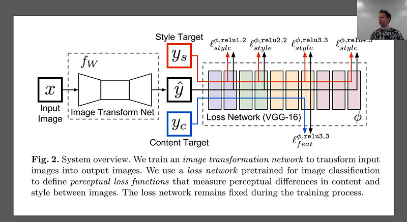
We are going to now turn the super resolution network into a style transfer network. And we’ll do this pretty quickly. We basically already have something. x is my input image and I’m going to have some loss function and I’ve got some neural net again. Instead of a neural net that does a whole a lot of compute and then does upsampling at the end, our input this time is just as big as our output. So we are going to do some downsampling first. Then our computer, and then our upsampling. So that’s the first change we are going to make — we are going to add some downsampling so some stride 2 convolution layers to the front of our network. The second is rather than just comparing yc and x are the same thing here. So we are going to basically say our input image should look like itself by the end. Specifically we are going to compare it by chucking it through VGG and comparing it at one of the activation layers. And then its style should look like some painting which we’ll do just like we did with the Gatys’ approach by looking at the Gram matrix correspondence at a number of layers. So that’s basically it. So that ought to be super straight forward. It’s really combining two things we’ve already done.
Bio: Hiromi Suenaga is a fast.ai student.
Related:
- An Introduction to Deep Learning for Tabular Data
- Quick Feature Engineering with Dates Using fast.ai
- An Overview of 3 Popular Courses on Deep Learning