 Beginners Ask “How Many Hidden Layers/Neurons to Use in Artificial Neural Networks?”
 Beginners Ask “How Many Hidden Layers/Neurons to Use in Artificial Neural Networks?”
By the end of this article, you could at least get the idea of how these questions are answered and be able to test yourself based on simple examples.
Beginners in artificial neural networks (ANNs) are likely to ask some questions. Some of these questions include what is the number of hidden layers to use? How many hidden neurons in each hidden layer? What is the purpose of using hidden layers/neurons? Is increasing the number of hidden layers/neurons always gives better results? I am pleased to tell we could answer such questions. To be clear, answering such questions might be too complex if the problem being solved is complicated. By the end of this article, you could at least get the idea of how these questions are answered and be able to test yourself based on simple examples.
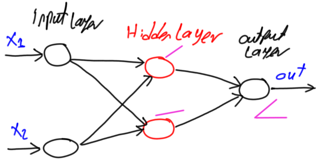
ANN is inspired by the biological neural network. For simplicity, in computer science, it is represented as a set of layers. These layers are categorized into three classes which are input, hidden, and output.
Knowing the number of input and output layers and number of their neurons is the easiest part. Every network has a single input and output layers. The number of neurons in the input layer equals the number of input variables in the data being processed. The number of neurons in the output layer equals the number of outputs associated with each input. But the challenge is knowing the number of hidden layers and their neurons.
Here are some guidelines to know the number of hidden layers and neurons per each hidden layer in a classification problem:
- Based on the data, draw an expected decision boundary to separate the classes.
- Express the decision boundary as a set of lines. Note that the combination of such lines must yield to the decision boundary.
- The number of selected lines represents the number of hidden neurons in the first hidden layer.
- To connect the lines created by the previous layer, a new hidden layer is added. Note that a new hidden layer is added each time you need to create connections among the lines in the previous hidden layer.
- The number of hidden neurons in each new hidden layer equals the number of connections to be made.
To make things clearer, let’s apply the previous guidelines for a number of examples.
Example 1
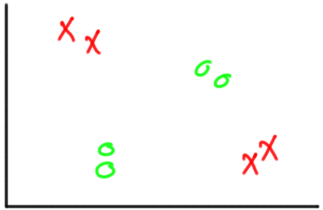
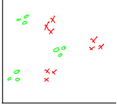
Let’s start with a simple example of a classification problem with two classes as shown in figure 1. Each sample has two inputs and one output that represents the class label. It is much similar to XOR problem.
Figure 1
The first question to answer is whether hidden layers are required or not. A rule to follow in order to determine whether hidden layers are required or not is as follows:
In artificial neural networks, hidden layers are required if and only if the data must be separated non-linearly.
Looking at figure 2, it seems that the classes must be non-linearly separated. A single line will not work. As a result, we must use hidden layers in order to get the best decision boundary. In such case, we may still not use hidden layers but this will affect the classification accuracy. So, it is better to use hidden layers.
Knowing that we need hidden layers to make us need to answer two important questions. These questions are:
- What is the required number of hidden layers?
- What is the number of the hidden neurons across each hidden layer?
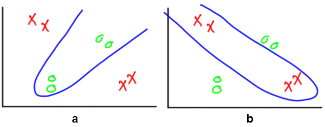
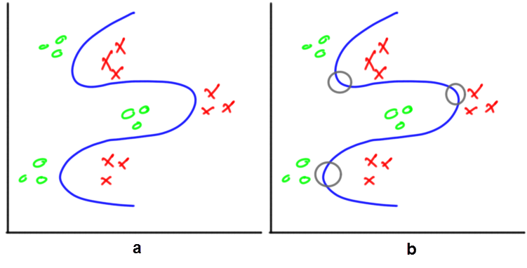
Following the previous procedure, the first step is to draw the decision boundary that splits the two classes. There is more than one possible decision boundary that splits the data correctly as shown in figure 2. The one we will use for further discussion is in figure 2(a).
Figure 2
Following the guidelines, next step is to express the decision boundary by a set of lines.
The idea of representing the decision boundary using a set of lines comes from the fact that any ANN is built using the single layer perceptron as a building block. The single layer perceptron is a linear classifier which separates the classes using a line created according to the following equation:
y = w_1*x_1 + w_2*x_2 + ⋯ + w_i*x_i + b
Where x_i is the input, w_i is its weight, b is the bias, and y is the output. Because each hidden neuron added will increase the number of weights, thus it is recommended to use the least number of hidden neurons that accomplish the task. Using more hidden neurons than required will add more complexity.
Returning back to our example, saying that the ANN is built using multiple perceptron networks is identical to saying that the network is built using multiple lines.
In this example, the decision boundary is replaced by a set of lines. The lines start from the points at which the boundary curve change direction. At such point, two lines are placed, each in a different direction.
Because there is just one point at which the boundary curve change direction as shown in figure 3 by a gray circle, then there will be just two lines required. In other words, there are two single layer perceptron networks. Each perceptron produces a line.
Figure 3
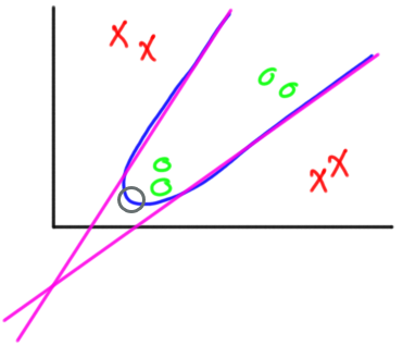
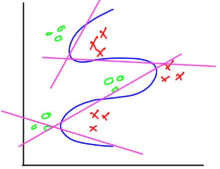
Knowing that there are just two lines required to represent the decision boundary tells us that the first hidden layer will have two hidden neurons.
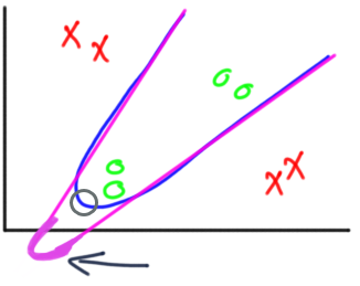
Up to this point, we have a single hidden layer with two hidden neurons. Each hidden neuron could be regarded as a linear classifier that is represented as a line as in figure 3. There will be two outputs, one from each classifier (i.e. hidden neuron). But we are to build a single classifier with one output representing the class label, not two classifiers. As a result, the outputs of the two hidden neurons are to be merged into a single output. In other words, the two lines are to be connected by another neuron. The result is shown in figure 4.
Fortunately, we are not required to add another hidden layer with a single neuron to do that job. The output layer neuron will do the task. Such neuron will merge the two lines generated previously so that there is only one output from the network.
Figure 4
After knowing the number of hidden layers and their neurons, the network architecture is now complete as shown in figure 5.
Figure 5
Example 2
Another classification example is shown in figure 6. It is similar to the previous example in which there are two classes where each sample has two inputs and one output. The difference is in the decision boundary. The boundary of this example is more complex than the previous example.
Figure 6
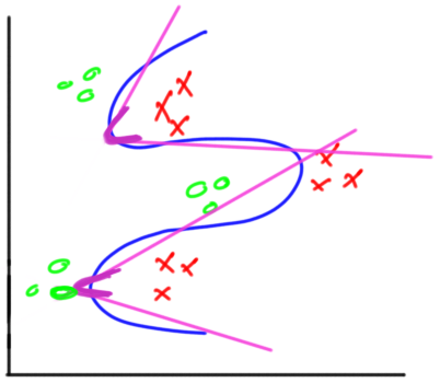
According to the guidelines, the first step is to draw the decision boundary. The decision boundary to be used in our discussion is shown in figure 7(a).
The next step is to split the decision boundary into a set of lines, where each line will be modeled as a perceptron in the ANN. Before drawing lines, the points at which the boundary change direction should be marked as shown in figure 7(b).
Figure 7
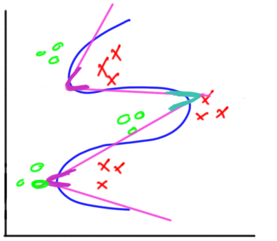
The question is how many lines are required? Each of top and bottom points will have two lines associated to them for a total of 4 lines. The in-between point will have its two lines shared from the other points. The lines to be created are shown in figure 8.
Because the first hidden layer will have hidden layer neurons equal to the number of lines, the first hidden layer will have 4 neurons. In other words, there are 4 classifiers each created by a single layer perceptron. At the current time, the network will generate 4 outputs, one from each classifier. Next is to connect these classifiers together in order to make the network generating just a single output. In other words, the lines are to be connected together by other hidden layers to generate just a single curve.
Figure 8
It is up to the model designer to choose the layout of the network. One feasible network architecture is to build a second hidden layer with two hidden neurons. The first hidden neuron will connect the first two lines and the last hidden neuron will connect the last two lines. The result of the second hidden layer. The result of the second layer is shown in figure 9.
Figure 9
Up to this point, there are two separated curves. Thus there are two outputs from the network. Next is to connect such curves together in order to have just a single output from the entire network. In this case, the output layer neuron could be used to do the final connection rather than adding a new hidden layer. The final result is shown in figure 10.
Figure 10
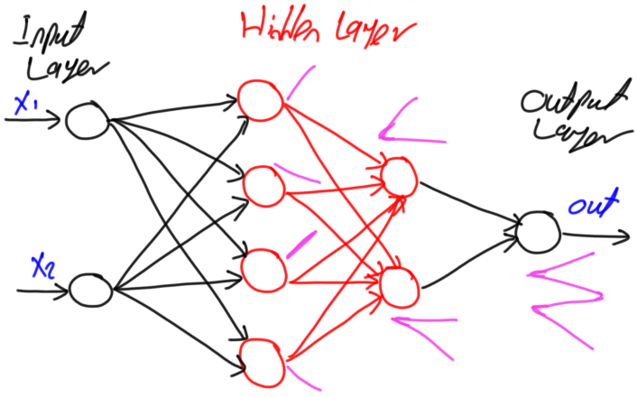
After network design is complete, the complete network architecture is shown in figure 11.
Figure 11
For more info,
Brief Introduction to Deep Learning + Solving XOR using ANNs
SlideShare: https://www.slideshare.net/AhmedGadFCIT/brief-introduction-to-deep-learning-solving-xor-using-anns
YouTube: https://www.youtube.com/watch?v=EjWDFt-2n9k
Bio: Ahmed Gad received his B.Sc. degree with excellent with honors in information technology from the Faculty of Computers and Information (FCI), Menoufia University, Egypt, in July 2015. For being ranked first in his faculty, he was recommended to work as a teaching assistant in one of the Egyptian institutes in 2015 and then in 2016 to work as a teaching assistant and a researcher in his faculty. His current research interests include deep learning, machine learning, artificial intelligence, digital signal processing, and computer vision.
Original. Reposted with permission.
Related:
- Avoid Overfitting with Regularization
- Building Convolutional Neural Network using NumPy from Scratch
- Derivation of Convolutional Neural Network from Fully Connected Network Step-By-Step