Derivation of Convolutional Neural Network from Fully Connected Network Step-By-Step

comments

In image analysis, convolutional neural networks (CNNs or ConvNets for short) are time and memory efficient than fully connected (FC) networks. But why? What are the advantages of ConvNets over FC networks in image analysis? How is ConvNet derived from FC networks? Where the term convolution in CNNs came from? These questions are to be answered in this article.

1. Introduction

 
Image analysis has a number of challenges such as classification, object detection, recognition, description, etc. If an image classifier, for example, is to be created, it should be able to work with a high accuracy even with variations such as occlusion, illumination changes, viewing angles, and others. The traditional pipeline of image classification with its main step of feature engineering is not suitable for working in rich environments. Even experts in the field won’t be able to give a single or a group of features that are able to reach high accuracy under different variations. Motivated by this problem, the idea of feature learning came out. The suitable features to work with images are learned automatically. This is the reason why artificial neural networks (ANNs) are one of the robust ways of image analysis. Based on a learning algorithm such as gradient descent (GD), ANN learns the image features automatically. The raw image is applied to the ANN and ANN is responsible for generating the features describing it.

2. Image Analysis using FC Network

 
Let’s see how ANN works with images and why CNN is efficient in its time and memory requirements W.R.T. the following 3x3 gray image in figure 1. The example given uses small image size and fewer number of neurons for simplicity.

Figure 1

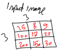
The inputs of the ANN input layer are the image pixels. Each pixel represents an input. Because the ANN works with 1D vectors, not 2D matrices, it is better to convert the above 2D image into a 1D vector as in figure 2.

Figure 2

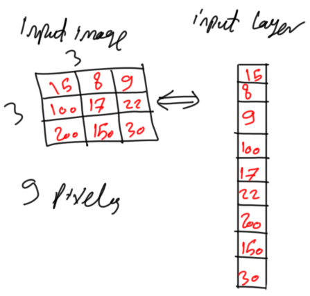
Each pixel is mapped to an element in the vector. Each element in the vector represented a neuron in ANN. Because the image has 3x3=9 pixels, then there will be 9 neurons in the input layer. Representing the vector as row or column doesn’t matter but ANN usually extends horizontally and each of its layers is represented as a column vector.

After preparing the input of the ANN, next is to add the hidden layer(s) that learns how to convert the image pixels into representative features. Assume that there is a single hidden layer with 16 neurons as in figure 3.

Figure 3

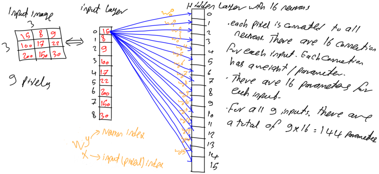
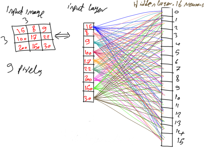
Because the network is fully connected, this means that each neuron in layer i is connected to all neurons in layer i-1. As a result, each neuron in the hidden layer is connected to all 9 pixels in the input layer. In other words, each input pixel is connected to the 16 neurons in the hidden layer where each connection has a corresponding unique parameter. By connecting each pixel to all neurons in the hidden layer, there will be 9x16=144 parameters or weights for such tiny network as shown in figure 4.

Figure 4

3. Large Number of Parameters

 
The number of parameters in this FC network seems acceptable. But this number highly increases as the number of image pixels and hidden layers increase.

For example, if this network has two hidden layers with a number of neurons of 90 and 50, then the number of parameters between the input layer and the first hidden layer is 9x90=810. The number of parameters between the two hidden layers is 90x50=4,500. The total number of parameters in such network is 810+4,500=5,310. This is a large number for such network. Another case of a very small image of size 32x32 (1,024 pixels). If the network operates with a single hidden layer of 500 neurons, there are a total of 1,024*500=512,000 parameter (weight). This is a huge number for a network with just single hidden layer working with a small image. There must be a solution to decrease such number of parameters. This is where CNN has a critical role. It creates a very large network but with less number of parameters than FC networks.

4. Neurons Grouping

 
The problem that makes the number of parameters gets very large even for small networks is that FC networks add a parameter between every two neurons in the successive layers. Rather than assigning a single parameter between every two neurons, a single parameter may be given to a block or group of neurons as in figure 5. The pixel with index 0 in figure 3 is connected to the first 4 neurons with indices (0, 1, 2, and 3) with 4 different weights. If the neurons are grouped in groups of 4 as in figure 5, then all neurons inside the same group will be assigned a single parameter.

Figure 5

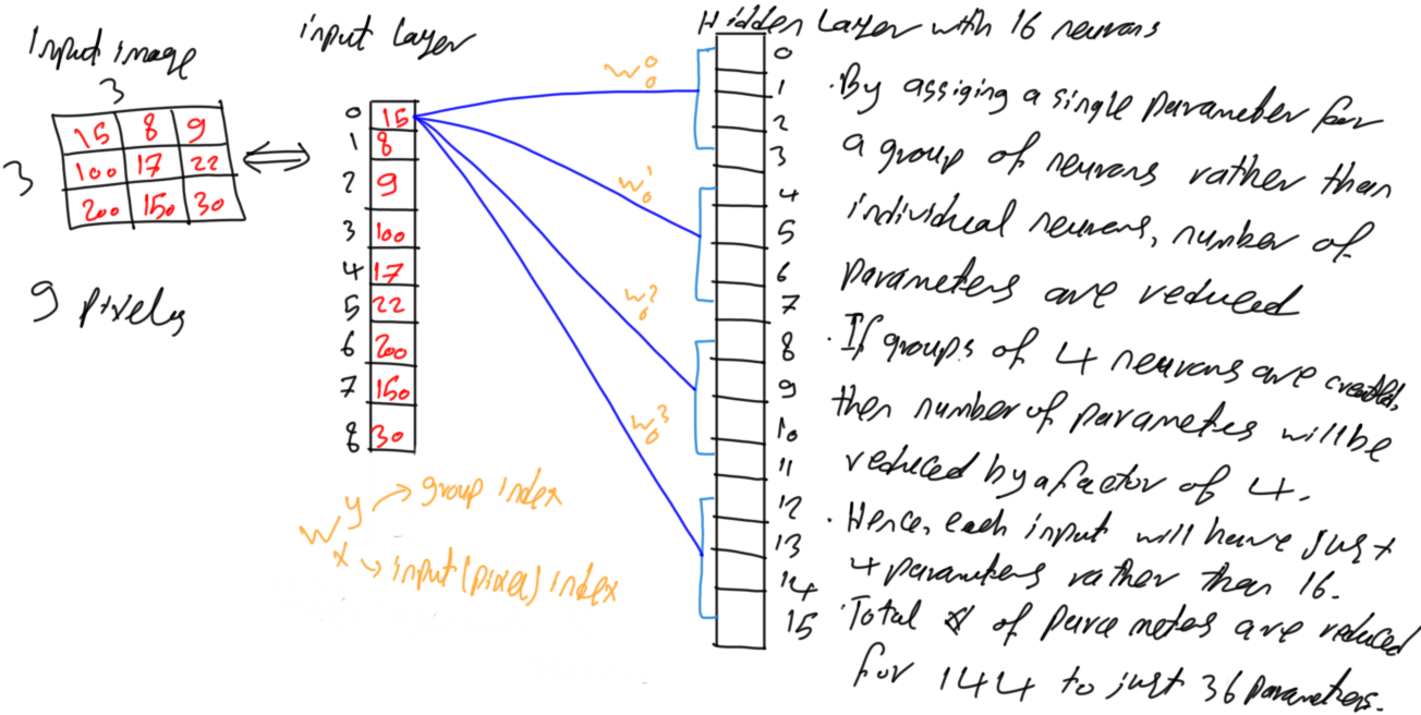
As a result, the pixel with index 0 in figure 5 will be connected to the first 4 neurons with the same weight as in figure 6. The same parameter is assigned to every 4 successive neurons. As a result, the number of parameters is reduced by a factor of 4. Each input neuron will have 16/4=4 parameters. The entire network will have 144/4=36 parameters. It is 75% reduction of the parameters. This is fine but still, it is possible to reduce more parameters.

Figure 6

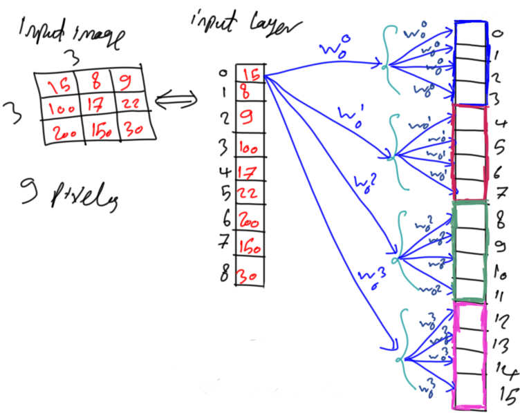
Figure 7 shows the unique connections from each pixel to the first neuron of each group. That is all missing connections are just a duplicate of the existing ones. Hypothetically, there is a connection from each pixel to each neuron in each group as in figure 4 because the network is still fully connected.

Figure 7

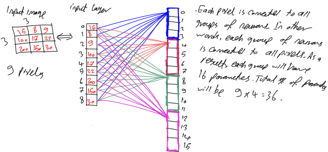
For making it simple, all connections are omitted except for the connections between all pixels to just the first neuron in the first group as shown in figure 8. It seems that each group is still connected to all 9 pixels and thus it will have 9 parameters. It is possible to reduce the number of pixels that such neuron is connected to.

Figure 8

5. Pixels Spatial Correlation

 
Current configuration makes each neuron accepts all pixels. If there is a function f(x1,x2,x3,x4) that accepts 4 inputs, that means the decision is to be taken based on all of these 4 inputs. If the function with just 2 inputs gives the same results as using all 4 inputs, then we do not have to use all of these 4 inputs. The 2 inputs giving the required results are sufficient. This is similar to the above case. Each neuron accepts all 9 pixels as inputs. If the same or better results will be returned by using fewer pixels, then we should go through it.

Usually, in image analysis, each pixel is highly correlated to pixels surrounding it (i.e. neighbors). The higher the distance between two pixels, the more they will be uncorrelated. For example, in the cameraman image shown in figure 9, a pixel inside the face is correlated to surrounding face pixels around it. But it is less correlated to far pixels such as sky or ground.

Figure 9
 

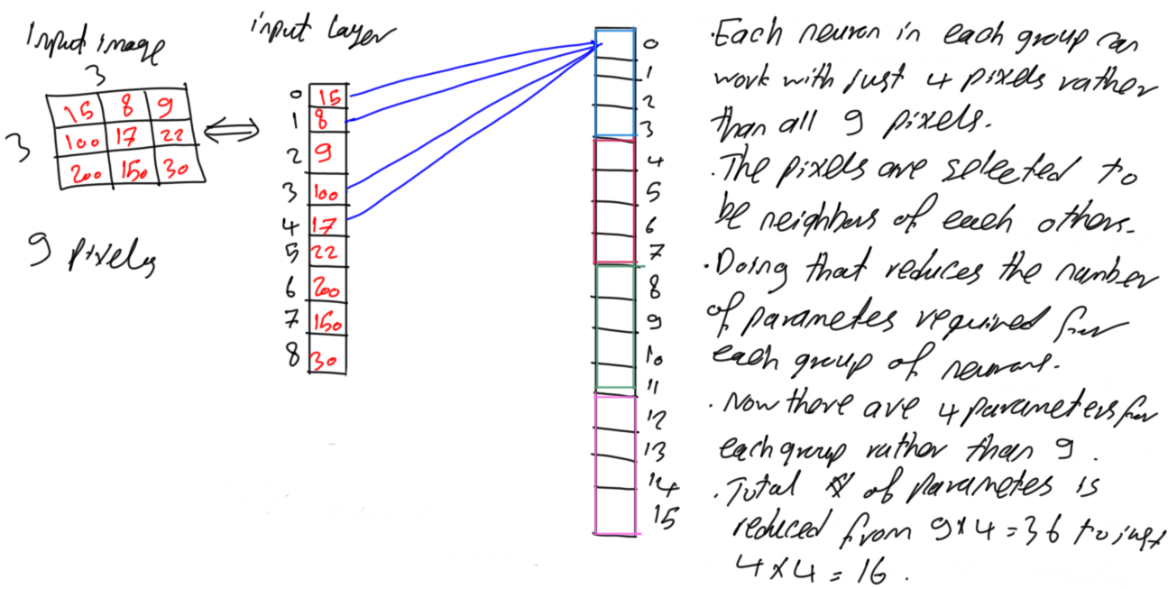
Based on such assumption, each neuron in the above example will accept just pixels that are spatially correlated to each other because working on all of them is reasonable. Rather than applying all 9 pixels to each neuron as input, it is possible to just select 4 spatially correlated pixels as in figure 10. The first pixel of index 0 in the column vector located at (0,0) in the image will be applied as an input to the first neuron with its 3 most spatially correlated pixels. Based on the input image, the 3 most spatially correlated pixels to that pixel are pixels with indices (0,1), (1,0), and (1,1). As a result, the neuron will accept just 4 pixels rather than 9. Because all neurons in the same group share the same parameters, then the 4 neurons in each group will have just 4 parameters rather than 9. As a result, the total number of parameters will be 4x4=16. Compared to the fully connected network in figure 4, there is a reduction of a 144-16=128 parameter (i.e. 88.89% reduction).

Figure 10

6. Convolution in CNN

 
At this point, the question of why CNN is more time and memory efficient than FC network is answered. Using fewer parameters allows the increase of a deep CNN with a huge number of layers and neurons which is not possible in FC network. Next is to get the idea of convolution in CNN.

Now there are just 4 weights assigned to all neurons in the same block. How will these 4 weights cover all 9 pixels? Let’s see how this works.

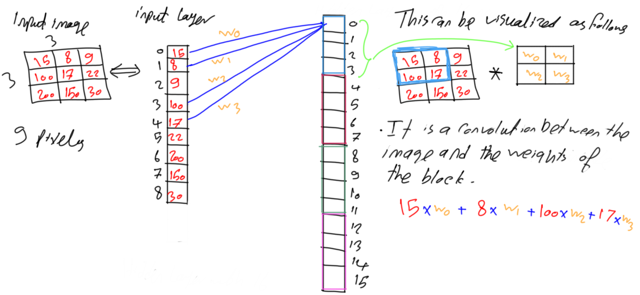
Figure 11 shows the previous network in figure 10 but after adding the weights labels to the connections. Inside the neuron, each of the 4 input pixels is multiplied by its corresponding weight. The equation is shown in figure 11. The four pixels and weights would be better visualized as matrices as in figure 11. The previous result will be achieved by multiplying the weights matrix to the current set of 4 pixels element-by-element. In practical, the size of the convolution mask should be odd such as 3x3. For being handled better, 2x2 mask is used in this example.

Figure 11

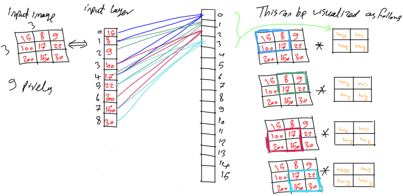
Moving to the next neuron of index 1, it will work with another set of spatially correlated pixels with the same weights used by the neuron with index 0. Also, neurons with indices 2 and 3 will work with other two sets of spatially correlated pixels. This is shown in figure 12. It seems that first neuron in the group starts from the top-left pixel and choose a number of pixels surrounding to it. The last neuron in the group works on the bottom-right pixel and its surrounding pixels. The in-between neurons are adjusted to select in-between pixels. Such behavior is identical to convolution. Convolution between the set of weights of the group and the image. This is why CNN has the term convolution.

Figure 12

The same procedure happens for the remaining groups of neurons. The first neuron of each group starts from the top-left corner and its surrounding pixels. The last neuron of each group works with the bottom-right corner and its surrounding pixels. The in-between neurons work on the in-between pixels.

7. References

 
Aghdam, Hamed Habibi, and Elnaz Jahani Heravi. Guide to Convolutional Neural Networks: A Practical Application to Traffic-Sign Detection and Classification. Springer, 2017.

 
Bio: Ahmed Gad received his B.Sc. degree with excellent with honors in information technology from the Faculty of Computers and Information (FCI), Menoufia University, Egypt, in July 2015. For being ranked first in his faculty, he was recommended to work as a teaching assistant in one of the Egyptian institutes in 2015 and then in 2016 to work as a teaching assistant and a researcher in his faculty. His current research interests include deep learning, machine learning, artificial intelligence, digital signal processing, and computer vision.

Original. Reposted with permission.

Related:

• Is Learning Rate Useful in Artificial Neural Networks?
• TensorFlow: Building Feed-Forward Neural Networks Step-by-Step
• Avoid Overfitting with Regularization