Introduction to Deep Learning with Keras
In this article, we’ll build a simple neural network using Keras. Now let’s proceed to solve a real business problem: an insurance company wants you to develop a model to help them predict which claims look fraudulent.
In this article, we’ll build a simple neural network using Keras. We’ll assume you have prior knowledge of machine learning packages such as scikit-learnand other scientific packages such as Pandas and Numpy.
Training an Artificial Neural Network
Training an artificial neural network involves the following steps:
- Weights are randomly initialized to numbers that are near zero but not zero.
- Feed the observations of your dataset to the input layer.
- Forward propagation (from left to right): neurons are activated and the predicted values are obtained.
- Compare predicted results to actual values and measure the error.
- Backward propagation (from right to left): weights are adjusted.
- Repeat steps 1–5
- One epoch is achieved when the whole training set has gone through the neural network.
Business Problem
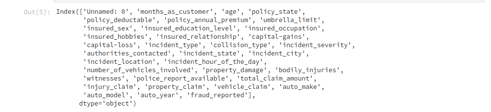
Now let’s proceed to solve a real business problem. An insurance company has approached you with a dataset of previous claims of their clients. The insurance company wants you to develop a model to help them predict which claims look fraudulent. By doing so you hope to save the company millions of dollars annually. This is a classification problem. These are the columns in our dataset.


Data Preprocessing
As in many business problems, the data provided will not be processed for us. We therefore have to prepare it in a way that our algorithm will accept it. We see from the dataset that we have some categorical columns. We need to convert these to zeros and ones so that our deep learning model will be able to understand them. Another thing to note is that we have to feed our dataset to the model as numpy arrays. Below we import the necessary packages and then load in our dataset.
import pandas as pd

import numpy as np

df = pd.read_csv(‘Datasets/claims/insurance_claims.csv’)
We then to convert the categorical columns to dummy variables.
In this case we use drop_first=True to avoid the dummy variable trap. For example, if you have a, b, c, d as categories then you can drop d as a dummy variable. This is because if something does not fall into either a, b, or c then it’s definitely in d. This is referred to as multicollinearity.
We use sklearn’s train_test_split to split the data into a training set and a test set.
from sklearn.model_selection import train_test_split
Next we make sure to drop the column we’re predicting to prevent it from leaking into the training set and the test set. We must avoid using the same dataset to train and test the model. We set .values at the end of the dataset in order to get the numpy arrays. This is the way our deep learning model will accept the data. This step is important because our machine learning model expects the data in form of arrays.
We then split the data into a training and test set. We use 0.7 of the data for training and 0.3 for testing.
X_train, X_test, y_train, y_test = train_test_split(X, y, test_size=0.3)
Next we have to scale our dataset using Sklearn’s StandardScaler. Due to the massive amounts of computations taking place in deep learning, feature scaling is compulsory. Feature scaling standardizes the range of our independent variables.
from sklearn.preprocessing import StandardScaler

sc = StandardScaler()

X_train = sc.fit_transform(X_train)

X_test = sc.transform(X_test)
Building the Artificial Neural Network(ANN)
The first thing we need to do is import Keras. By default, Keras will use TensorFlow as its backend.
import keras
Next we need to import a few modules from Keras. The Sequential module is required to initialize the ANN, and the Dense module is required to build the layers of our ANN.
from keras.models import Sequential

from keras.layers import Dense
Next we need to initialize our ANN by creating an instance of Sequential. The Sequential function initializes a linear stack of layers. This allows us to add more layers later using the Dense module.
classifier = Sequential()
Adding input layer (First Hidden Layer)
We use the add method to add different layers to our ANN. The first parameter is the number of nodes you want to add to this layer. There is no rule of thumb as to how many nodes you should add. However a common strategy is to choose the number of nodes as the average of nodes in the input layer and the number of nodes in the output layer.
Say for example you had five independent variables and one output. Then you would take the sum of that and divide by two, which is three. You can also decide to experiment with a technique called parameter tuning. The second parameter, kernel_initializer, is the function that will be used to initialize the weights. In this case, it will use a uniform distribution to make sure that the weights are small numbers close to zero. The next parameter is the activation function. We use the Rectifier function, shortened as relu. We mostly use this function for the hidden layer in ANN. The final parameter is input_dim, which is the number of nodes in the input layer. It represents the number of independent variables.
classsifier.add(
        Dense(3, kernel_initializer = ‘uniform’,
              activation = ‘relu’, input_dim=5))
Adding Second Hidden Layer
Adding the second hidden layer is similar to adding the first hidden layer.
classsifier.add(
      Dense(3, kernel_initializer = ‘uniform’,
            activation = ‘relu’))
We don’t need to specify the input_dim parameter because we have already specified it in the first hidden layer. In the first hidden layer we specified this in order to let the layer know how many input nodes to expect. In the second hidden layer the ANN already knows how many input nodes to expect so we don’t need to repeat ourselves.
Adding the output layer
classifier.add(
     Dense(1, kernel_initializer = ‘uniform’,
           activation = ‘sigmoid’))
We change the first parameter because in our output node we expect one node. This is because we are only interested in knowing whether a claim was fraudulent or not. We change the activation function because we want to get the probabilities that a claim is fraudulent. We do this by using the Sigmoid activation function. In case you’re dealing with a classification problem that has more than two classes (i.e. classifying cats, dogs, and monkeys) we’d need to change two things. We ‘d change the first parameter to 3 and change the activation function to softmax. Softmax is a sigmoid function applied to an independent variable with more than two categories.