Introduction to Deep Learning with Keras

comments

Compiling the ANN

classifier.compile(optimizer= ‘adam’,
                  loss = ‘binary_crossentropy’,
                  metrics = [‘accuracy’])

Compiling is basically applying a stochastic gradient descent to the whole neural network. The first parameter is the algorithm you want to use to get the optimal set of weights in the neural network. The algorithm used here is a stochastic gradient algorithm. There are many variants of this. A very efficient one to use is adam. The second parameter is the loss function within the stochastic gradient algorithm. Since our categories are binary we use the binary_crossentropy loss function. Otherwise we would have used categorical_crossentopy. The final argument is the criterion we’ll use to evaluate our model. In this case we use the accuracy.

Fitting our ANN to the training set

classifier.fit(X_train, y_train, batch_size = 10, epochs = 100)

X_train represents the independent variables we’re using to train our ANN, and y_train represents the column we’re predicting. Epochs represents the number of times we’re going to pass our full dataset through the ANN. Batch_size is the number of observations after which the weights will be updated.

Predicting using the training set

y_pred = classifier.predict(X_test)

This will show us the probability of a claim being fraudulent. We then set a threshold of 50% for classifying a claim as fraudulent. This means that any claim with a probability of 0.5 or more will be classified as fraudulent.

y_pred = (y_pred > 0.5)

This way the insurance firm can be able to first track claims that are not suspicious and then take more time evaluating claims flagged as fraudulent.

Checking the confusion matrix

from sklearn.metrics import confusion_matrix

cm = confusion_matrix(y_test, y_pred)

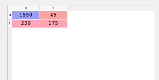
The confusion matrix can be interpreted as follows. Out of 2000 observations, 1550 + 175 observations were correctly predicted while 230 + 45 were incorrectly predicted. You can calculate the accuracy by dividing the number of correct predictions by the total number of predictions. In this case (1550+175) / 2000, which gives you 86%.

Making a single Prediction

 
Let’s say the insurance company gives you a single claim. They’d like to know if the claim is fraudulent. What would you do to find out?

new_pred = classifier.predict(sc.transform(np.array([[a,b,c,d]])))

where a,b,c,d represents the features you have.

new_pred = (new_prediction > 0.5)

Since our classifier expects numpy arrays, we have to transform the single observation into a numpy array and use the standard scaler to scale it.

Evaluating our ANN

 
After training the model one or two times, you’ll notice that you keep getting different accuracies. So you’re not quite sure which one is the right one. This introduces the bias variance trade off. In essence, we’re trying to train a model that will be accurate and not have too much variance of accuracy when trained several times. To solve this problem we use the K-fold cross validation with K equal to 10. This will split the training set into 10 folds. We’ll then train our model on 9 folds and test it on the remaining fold. Since we have 10 folds, we’re going to do this iteratively through 10 combinations. Each iteration will gives us its accuracy. We’ll then find the mean of all accuracies and use that as our model accuracy. We also calculate the variance to ensure that it’s minimal.

Keras has a scikit learn wrapper (KerasClassifier) that enables us to include K-fold cross validation in our keras code.

from keras.wrappers.scikit_learn import KerasClassifier

Next we import the k-fold cross validation function from scikit_learn

from sklearn.model_selection import cross_val_score

The KerasClassifier expects one of its arguments to be a function, so we need to build that function.The purpose of this function is to build the architecture of our ANN.

This function will build the classifier and return it for use in the next step. The only thing we have done here is wrap our previous ANN architecture in a function and return the classifier.

We then create a new classifier using K-fold cross validation and pass the parameter build_fn as the function we just created above. Next we pass the batch size and the number of epochs, just like we did in the previous classifier.

classiifier = KerasClassifier(build_fn = make_classifier,
                            batch_size=10, nb_epoch=100)

To apply the k-fold cross validation function we can use scikit-learn’s cross_val_score function. The estimator is the classifier we just built with make_classifier and n_jobs=-1 will make use of all available CPUs. cv is the number of folds and 10 is a typical choice. The cross_val_score will return the ten accuracies of the ten test folds used in the computation.

accuracies = cross_val_score(estimator = classifier,
                             X = X_train,
                             y = y_train,
                             cv = 10,
                             n_jobs = -1)

To obtain the relative accuracies we get the mean of the accuracies.

mean = accuracies.mean()

The variance can be obtained as follows:

variance = accuracies.var()

The goal is to have a small variance between the accuracies.

Fighting Overfitting

 
Overfitting in machine learning is what happens when a model learns the details and noise in the training set such that it performs poorly on the test set. This can be observed when we have huge differences between the accuracies of the test set and training set or when you observe a high variance when applying k-fold cross validation. In artificial neural networks, we counteract this using a technique called dropout regularization. Dropout regularization works by randomly disabling some neurons at each iteration of the training to prevent them from being too dependent on each other.

In this case we apply the dropout after the first hidden layer and after the second hidden layer. Using a rate of 0.1 means that 1% of the neurons will be disabled at each iteration. It is advisable to start with a rate of 0.1. However you should never go beyond 0.4 because you will now start to get underfitting.

Parameter Tuning

 
Once you obtain your accuracy you can tune the parameters to get a higher accuracy. Grid Search enable us to test different parameters in order to obtain the best parameters.

The first step here is to import the GridSearchCV module from sklearn.

from sklearn.model_selection import GridSearchCV

We also need to modify our make_classifier function as follows. We create a new variable called optimizer that will allow us to add more than one optimizer in our params variable.

We’ll still use the KerasClassifier, but we won’t pass the batch size and number of epochs since these are the parameters we want to tune.

classifier = KerasClassifier(build_fn = make_classifier)

The next step is to create a dictionary with the parameters we’d like to tune — in this case the batch size, the number of epochs, and the optimizer function. We still use adam as an optimizer and add a new one called rmsprop. The Keras documentation recommends rmsprop when dealing with Recurrent Neural Networks. However we can try it for this ANN to see if it gives us a better result.

params = {
    'batch_size':[20,35],

    'nb_epoch':[150,500],

    'Optimizer':['adam','rmsprop']
}

We then use Grid Search to test these parameters. The grid search function expects our estimator, the parameters we just defined, the scoring metric and the number of k-folds.

grid_search = GridSearchCV(estimator=classifier,
                           param_grid=params,
                           scoring=’accuracy’,
                           cv=10)

Like in previous objects we need to fit our training set.

grid_search = grid_search.fit(X_train,y_train)

We can get the best selection of parameters using best_params from the grid search object. Likewise we use the best_score_ to get the best score.

best_param = grid_search.best_params_

best_accuracy = grid_search.best_score_

It’s important to note that this process will take a while as it searches for the best parameters.

Conclusion

 
Artificial Neural Networks are just one type of deep neural network. There are other networks such Recurrent Neural Networks (RNN), Convolutional Neural Network (CNN), and Boltzmann machine. RNNs can predict if the price of a stock will go up or down in the future. CNNs are used in computer vision — recognizing cats and dogs in a set of images or recognizing the presence of cancer cells in a brain image. Boltzmann machines are used in programming recommender systems. Maybe we can cover one of these neural networks in the future.

Cheers.

 
Bio: Derrick Mwiti is a data analyst, a writer, and a mentor. He is driven by delivering great results in every task, and is a mentor at Lapid Leaders Africa.

Original. Reposted with permission.

Related:

• The Keras 4 Step Workflow
• 7 Steps to Mastering Deep Learning with Keras
• Beginner Data Visualization & Exploration Using Pandas