 Common mistakes when carrying out machine learning and data science
 Common mistakes when carrying out machine learning and data science
We examine typical mistakes in Data Science process, including wrong data visualization, incorrect processing of missing values, wrong transformation of categorical variables, and more. Learn what to avoid!
By Jekaterina Kokatjuhha, Research Engineer at Zalando.
This is part two of this series, find part one here - How to build a data science project from scratch.
After scraping or getting the data, there are many steps to accomplish before applying a machine learning model.
You need to visualize each of the variables to see distributions, find the outliers, and understand why there are such outliers.
What can you do with missing values in certain features?
What would be the best way to convert categorical features into numerical ones?
There are many such questions, but I will give some details on the ones where the majority of beginners encounter mistakes.
1. Visualization
Firstly, you should visualize the distribution of the continuous features to get a feeling if there are many outliers, what the distribution would be, and if it makes sense.
There are many ways to visualize it, for example box plots, histograms, cumulative distribution functions, and violin plots. However, one should pick the plot that will give the most information about the data.
To see the distribution (if it is normal, or bimodal), the histograms will be the most helpful. Although histograms are a good starting point, the box plots might be superior in identifying the number of outliers and seeing where the median quartiles lie.
Based on the plots, the most interesting question would be: do you see what you expected to see? Answering this question will help you either in finding insights or finding bugs in the data.
To get inspired and understand what plot will give the most value, I frequently referred to the Python’s seaborn gallery. Another good source of inspiration for the visualization and finding insights are kernels on Kaggle. Here is my kaggle kernel of the in-depth visualization of the titanic dataset.
In the context of rental prices, I plotted the histograms of each continuous feature and expected to see a long right tail in the distribution of the rent without bills and total area.
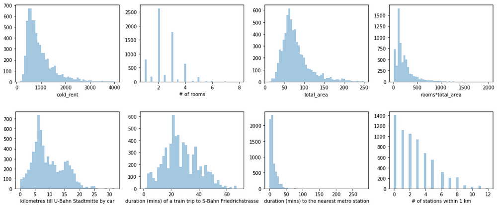
Histograms of continuous features
Box plots helped me see the number of outliers for each of the features. In fact, most of the outliers apartments based on the rent without bills were either the ateliers for the small shops with more than 200m2 or the student dormitories with very low rent.
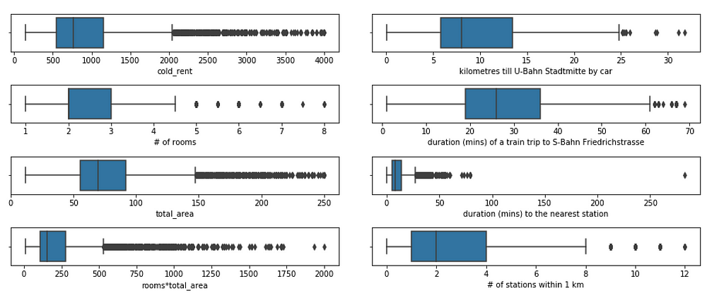
Boxplots of continuous features
2. Do I impute the values based on the whole dataset?
Sometimes there will be missing values, due to various reasons. If we exclude every observation with at least one missing value, we can end up with a very reduced dataset.
There are many ways of imputing the values, mean, or median. It is up to you how to do it but make sure to calculate the imputation statistics only on the training data to avoid data leakage of your test set.
In the rental data, I also extracted a description of the apartment. Whenever the quality, condition, or type of apartment was missing, I would impute it from the description if the description contained this information.
3. How do I transform categorical variables?
Some algorithms, depending on the implementation, wouldn’t work directly with the categorical data, so one would need to somehow transform them into numerical values.
There are many ways of transforming categorical variables into numerical features, such as Label Encoder, One Hot Encoding, bin encoding, and hashing encoding. However, most people use the Label Encoding incorrectlywhen the One Hot Encoding should have been used instead.
Assume, in our rental data, that we have an apartment-type column with the following values: [ground floor, loft, maisonette, loft, loft, ground floor]. LabelEncoder can turn this into [3,2,1,2,2,1], introducing ordinality, which means that ground_floor >loft > maisonette. For some algorithms like decision trees, and its deviations, this type of encoding for this feature would be fine, but applying regressions and SVM might not make that much sense.
In the rental price dataset, the condition is encoded as follows:
- new:1
- renovated:2
- needs renovation: 3
and the quality as:
- Luxus:1
- better than normal: 2
- normal: 3
- simple: 4
- unknown: 5
4. Do I need to standardize variables?
Standardization brings all continuous variables to the same scale, meaning if one variable has values from 1K to 1M and another from 0.1 to 1, after standardization they will have the same range.
L1 or L2 regularizations are the common way of reducing overfitting and can be used within many regression algorithms. However, it is important to apply feature standardization before L1 or L2.
The rental price is in Euros so the fitted coefficient would be approximately 100 times larger than the fitted coefficient if the price was in cents. L1 and L2 penalize the larger coefficients more, meaning it will penalize the features in smaller scales more. To prevent this, the features should be standardized before applying L1 or L2.
Another reason to standardize is that if you or the your algorithm use gradient descent, gradient descent converges much faster with feature scaling.
5. Do I need to derive the logarithm of the target variable?
It took me a while to understand that there is no universal answer.
It depends on many factors:
- whether you want fractional or absolute error
- which algorithm you use
- what residual plots and changes in the metrics tell you
In regression, firstly pay attention to the residual plots and the metric. Sometimes the logarithmization of the target variable leads to a better model and the results of the model would still be easy to understand. However, there are still other transformations that could be of interest, such as to taking the square root.
There are many answers on Stack Overflow regarding this question, and I think Residual Plots and RMSE on raw and log target variable explains it very well.
For the rental data, I derived the logarithm of the price as the residual plots looked a bit better.
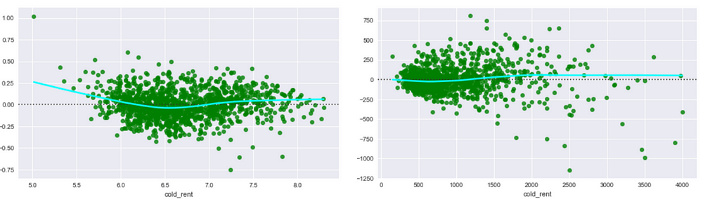
Residual plots of the logarithms (left) and untransformed data (right) of rent not including the bills variable. The right plot exhibits “heteroscedasticity” — the residuals get larger as the prediction moves from small to large.
Some more important stuff
Some algorithms, such as regressions, will suffer from collinearities in the data because the coefficients become very unstable (more math). SVM might or might not suffer from collinearity due to the choice of kernel.
Decision-based algorithms will not suffer from multicollinearity as they could use features interchangeably in different trees without it affecting the performance. However, the interpretation of feature importance then gets more difficult as the correlated variable may not appear to be as important as it is.
Machine learning
After you have familiarized yourself with data and cleaned out the outliers, it is the perfect time to get the hang of machine learning. There are many algorithms you could use for this supervised machine learning.
There were three different algorithms I wanted to explore, comparing characterstics such as performance differences and speed. These three were gradient boosted trees with different implementations (XGBoost and LightGMB), Random Forest (FR, scikit-learn) and 3-layer Neuronal Networks (NN, Tensorflow). I selected RMSLE (root mean squared logarithm error) to be the metric for the optimization of the process. I used RMSLE because I derived the logarithm of the target variable.
XGBoost and LigthGBM performed comparably, RF slightly worse, whereas NN was the worst.

Performance (RMSLE) of the algorithms on the test set.
Decision tree-based algorithms are very good at interpreting features. For example, they produce a feature importance score.
Feature importance: finding the drivers of the rental price
After fitting a decision tree-based model, you can see what features are the most valuable for the price prediction.
Feature importance provides a score that indicates how informative each feature was in the construction of the decision trees within the model. One of the ways to calculate this score is to count how many times a feature is used to split the data across all trees. This score can be computed in different ways.
Feature importance can reveal other insights about the main price drivers.
For the rental price prediction, it isn’t surprising that total area is the most important driver of the price. Interestingly, some features that were engineered with external API are also in the top most important features.
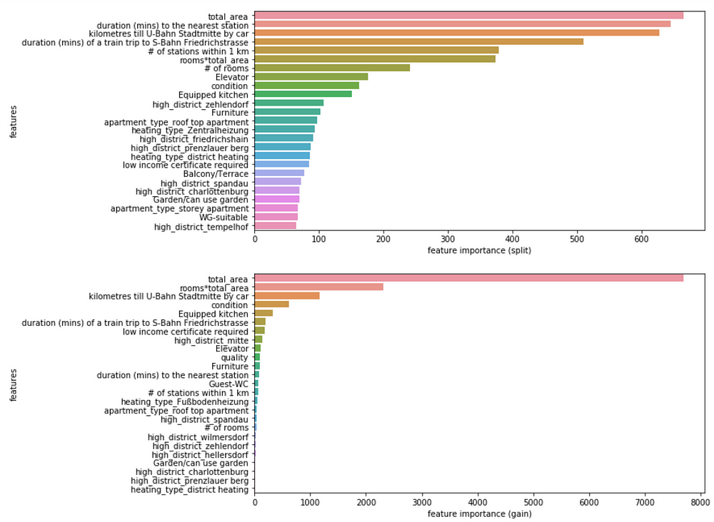
Feature importance calculated by split (above) and by gain (below)
However, as mentioned in “Interpretable Machine Learning with XGBoost”, there can be inconsistencies in feature importance depending on the attribution option. The author of the linked blogpost, and SHAP NIPS paper, proposes a new way of calculating feature importance that will be both accurate and consistent. This uses the shap Python library. SHAP values represent the responsibility of a feature for a change in the model output.
The output of the analysis on the rental price data is shown in the figure below.
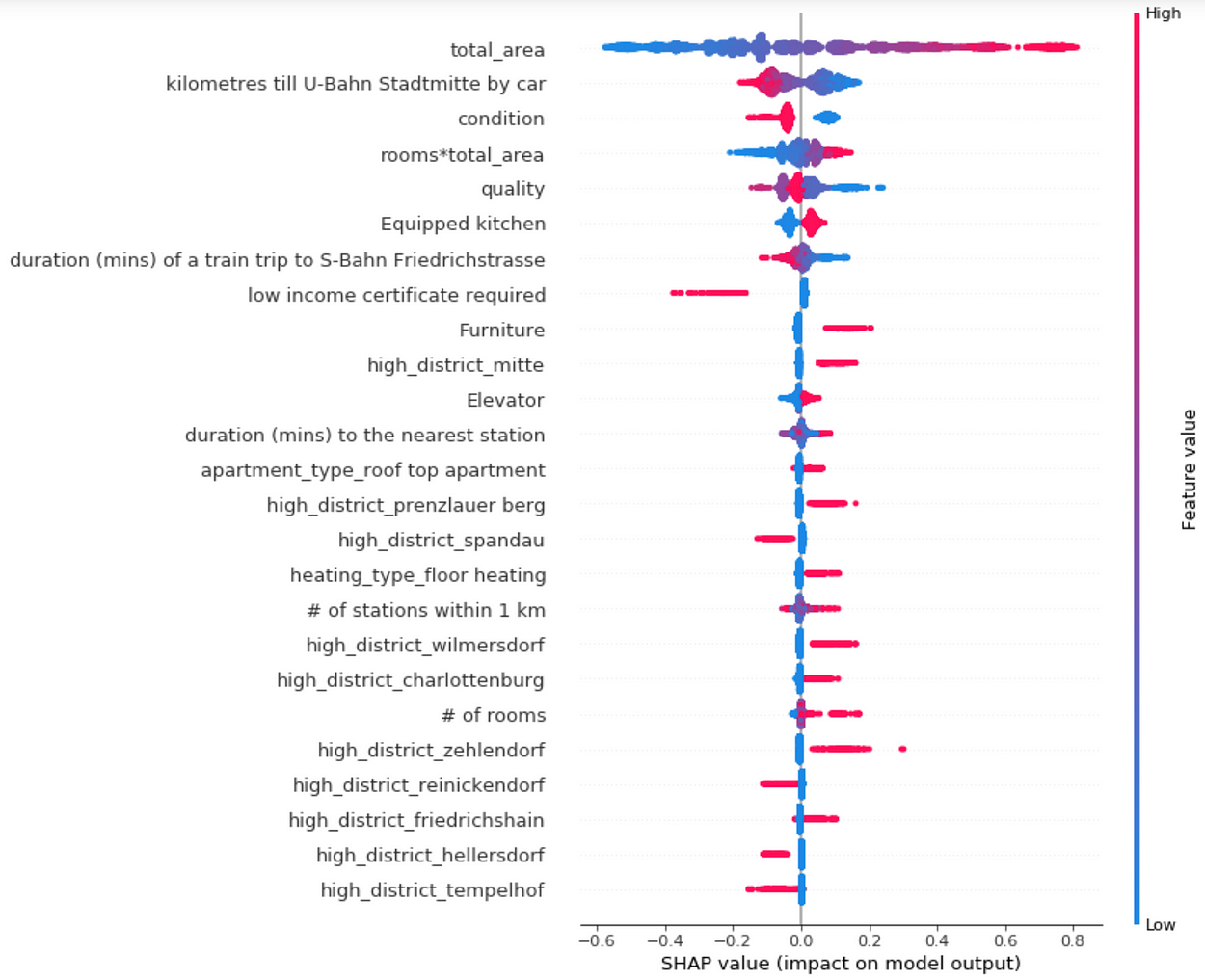
Each apartment has one dot on each row. The x position of the dot is the impact of that feature on the model’s prediction for the customer, and the color of the dot represents the value of that feature for the apartment
The figure incorporates a lot of valuable information (features are sorted by mean (|Tree SHAP|)). Small disclaimer: data is from the beginning of 2018; the district can evolve and therefore the price-dependent factors could change.
- the proximity to the city center (kilometers till U-Bahn Stadtmitte by car and duration of a train trip to S-Bahn Friedrichstrasse) increases the predicted rental apartment price
- total area as the strongest driver of the rental price
- if the apartment owner requires you to have a low income certificate (WBS in German), the predicted price is lower
- renting an apartment in these districts would also increase the rental price: Mitte, Prenzlauer Berg, Wilmersdorf, Charlottenburg, Zehlendorf and Friedrichshain.
- districts with lower prices would be: Spandau, Tempelhof, Wedding and Reinickendorf
- obviously, an apartment in better condition — the lower value is the better — of better quality — the lower value is better — with furniture, a built-in kitchen, and elevator will cost more
Interesting are the impacts of following features:
- duration to the nearest metro station
- number of stations within 1 km.
Duration to the nearest metro station:
It seems that, for some apartments, the high value of this feature indicates the higher price. The reason for this is that these apartments are situated in very wealthy residential areas outside of Berlin.
One can also see that the proximity to the metro station has two directions: it lowers and it increases the price for some apartments. The reason could be that the apartments that are very close to metro station would also suffer from underground noise or vibrations caused by trains but, on the other hand, they would be well-connected to the public transportation. However, one could investigate a bit more into this feature as it shows the proximity only to the nearest metro stations and not tram/bus stations.
Number of stations within 1 km:
The same applies to the number of stations within one kilometer from the apartment. Many metro stations around would, in general, increase the rental price. However, it also had a negative effect — more noise.
Ensemble averaging
After playing around with different models and comparing performance, you could just combine the results of each of the model and build an ensemble!
Bagging is the machine learning ensemble model that utilizes the predictions of several algorithms to calculate the final aggregated predictions. It is designed to prevent overfitting and reduces the variance of the algorithms.
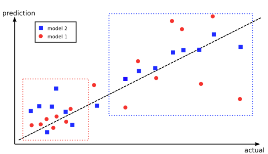
Advantage of using ensembles: The red model performs better in the lower left box, however, the blue model performs better in the upper right box. By combining the predictions from both models, it could improve the overall performance. Fig taken from here.
As I already had predictions from the above mentioned algorithms, I combined all four models in all possible ways and picked the seven best single and ensemble models based on the RMSLE of the validation set.
Then the RMSLE of those seven models was calculated on the test set.
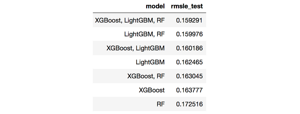
Test RMSLE of the algorithms.
The ensemble of three decision-tree based algorithms performed the best compared to each single model.
You could also produce a weighted ensemble, assigning more weight to a better single model. The reasoning behind it is that other models could overrule the best model only if they collectively agree on an alternative.
In reality, one would never know if an averaged ensemble would be better than the single model without just trying it out.
Stacked models
An averaged or weighted ensemble is not the only way to combine the predictions of different models. You could also stack the models in very different ways!
The idea behind stacked models is to create several base models and a meta model on top of the results from the base models in order to produce final predictions. However, it is not so obvious how to train the meta model because it can be biased towards the best of the base models. A very good explanation of how to do it correctly can be found in the post “Stacking models for improved predictions”.
For the rental price case, stacked models didn’t improve the RMSLE at all — they even increased the metrics. There might be several reasons for this — either I coded it incorrectly ;) or there was just too much noise introduced by stacking.
If you want to explore more of the ensemble and stacked model articles, the Kaggle Ensemble Guide explains many different kinds of ensembling with the performance comparison and referrals on how such stacked models got to the top of Kaggle’s competitions.
Final thoughts
- listen to what people talk about around you; their complaining can serve as a good starting point for solving something big
- let people find their own insights by providing interactive dashboards
- don’t restrict yourself to common feature engineering as multiplying two variables. Try to find additional sources of data or explanations
- try out ensembles and stacked models as those methods could improve the performance
And please, provide the date of the data you display!
Sources of figures:
https://www.pinterest.de/minimalcouture/paris-apartments/
https://www.theodysseyonline.com/the-struggles-of-moving-into-your-first-apartment
https://www.fashionbeans.com/content/the-worlds-10-smallest-apartments-are-downright-shocking/
Bio: Jekaterina Kokatjuhha is a Research Engineer at Zalando, focusing on scalable machine learning for fraud prediction.
Original. Reposted with permission.
Resources:
- On-line and web-based: Analytics, Data Mining, Data Science, Machine Learning education
- Software for Analytics, Data Science, Data Mining, and Machine Learning
Related:
- Data Science Projects Employers Want To See: How To Show A Business Impact
- The 5 Common Mistakes That Lead to Bad Data Visualization
- 10 Mistakes to Avoid When Adopting Advanced Analytics