How to do Everything in Computer Vision
The many standard tasks in computer vision all require special consideration: classification, detection, segmentation, pose estimation, enhancement and restoration, and action recognition. Let me show you how to do everything in Computer Vision with Deep Learning!
Want to do Computer Vision? Deep Learning is the way to go these days. Large scale datasets plus the representational power of deep Convolutional Neural Networks (CNNs) make for super accurate and robust models. Only one challenge still remains: how to design your model.
With a field as broad and complex as computer vision, the solution isn’t always clear. The many standard tasks in computer vision all require special consideration: classification, detection, segmentation, pose estimation, enhancement and restoration, and action recognition. Although the state-of-the-art networks used for each of them exhibit common patterns, they’ll all still need their own unique design twist.
So how can we build models for all of those different tasks?
Let me show you how to do everything in Computer Vision with Deep Learning!
Classification
The most well known of them all! Image classification networks start with an input of fixed size. The input image can have any number of channels, but is usually 3 for an RGB image. When you design your network, the resolution can technically be any size as long as it is large enough to support the amount of downsampling you will do throughout the network. For example, if you downsample 4 times within the network, then your input needs to at least be 4² = 16 x 16 pixels in size.
As you go deeper into the network the spatial resolution will decrease as we try to squeeze all of that information and get down to a 1-dimensional vector representation. To insure that the network always has the capacity to carry forward all of the information it extracts, we increase the number of feature maps proportionally to the depth to accommodate the reduction in spatial resolution. I.e we are losing spatial information in our downsampling process, and to accommodate the loss we expand our feature maps to increase our semantic information.
After a certain amount of downsampling that you have selected, the feature maps are vectorized and fed into a series of fully connected layers. The last layer has as many outputs as there are classes in your dataset.

Object Detection
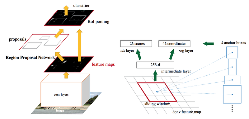
Object detectors come in 2 flavours: one-stage and two-stage. Both of them start out with “anchor boxes”; these are default bounding boxes. Our detector is going to predict the difference between those boxes and the ground-truth, rather than predicting the boxes directly.
In a two-stage detector we naturally have two networks: a box proposal network and a classification network. The box proposal network proposes coordinates for bounding boxes where it thinks there is a high likelihood that objects are there; again these are relative to the anchor boxes. The classification network then takes each of these bounding boxes and classifies the potential object that lies within it.
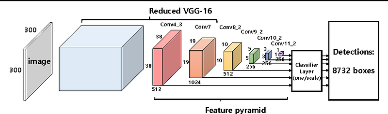
In a one-stage detector, the proposal and classifier networks are fused into one single stage. The network directly predicts both the bounding box coordinates and the class which resides within that box. Because the two stages are fused together, one-stage detectors tend to be faster than two-stage. But the two-stage detectors have higher accuracy due to the separation of the two tasks.
Segmentation
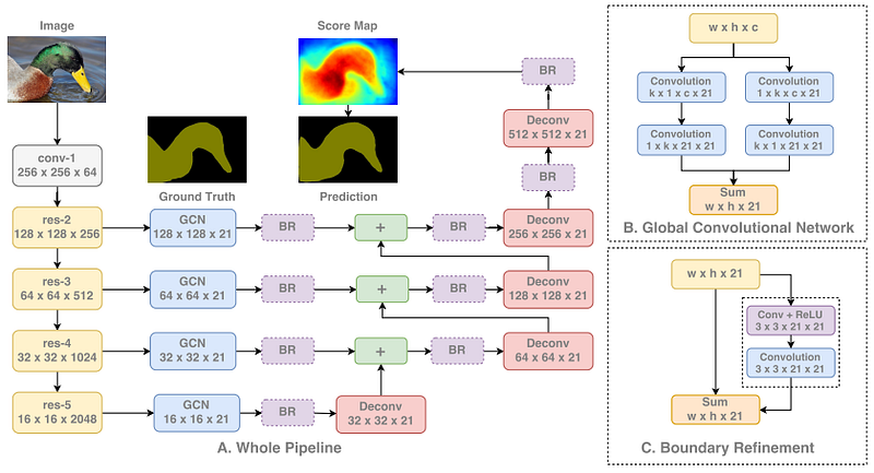
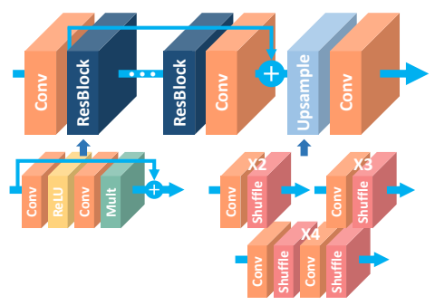
Segmentation is one of the more unique tasks in computer vision in that the networks need to learn both low- and high-level information. Low-level information to accurately segment each area and object in the image by the pixel, and high-level information to directly classify those pixels. This leads to networks being designed to combine the information from earlier layers and high-resolution (low-level spatial information) with deeper layers and low-resolution (high-level semantic information).
As we can see below, we first run our image through a standard classification network. We then extract features from each stage of the network, thus using information from a range of low-to-high. Each information level is processed independently before combining them all together in turn. As the information is combined, we upsample the feature maps to eventually get to the full image resolution.
To learn more details about how segmentation with deep learning works, check out this article.
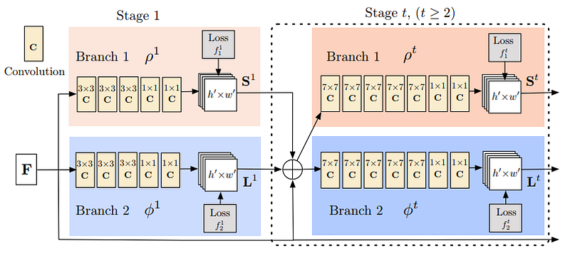
Pose Estimation
Pose estimation models need to accomplish 2 tasks: (1) detect keypoints in an image for each body part (2) find out how to properly connect those keypoints. This is done in three stages:
(1) Extract features from the image using a standard classification network
(2) Given those features, train a sub-network to predict a set of 2D heatmaps. Each heatmap is associated with a particular keypoint and contains confidence values for each image pixel about whether a keypoint likely exists there or not
(3) Again given the features from the classification network, we train a sub-network to predict a set of 2D vector fields, where each vector field encodes the degree of association between the keypoints. Keypoints with high association are then said to be connected.
Training the model in this way with the sub-networks will jointly optimise detecting the keypoints and connecting them together.
Enhancement and Restoration
Enhancement and restoration networks are their own unique beast. We don’t do any downsampling with these since what we are really concerned about is high-pixel / spatial accuracy. Downsampling would really kill this information since it would reduce how many pixels we have for spatial accuracy. Instead, all processing is done at the full image resolution.
We begin by passing the image we want to enhance / restore to our network without any modification, at full-resolution. The network simply consists of a stack of many convolutions and activation function. These blocks are typically inspired and occasionally direct copies of those originally developed for image classification such as Residual Blocks, Dense Blocks, Squeeze Excitation Blocks, etc. There is no activation function on the last layer, not even sigmoid or softmax, since we want to predict the image pixels directly and do not require any probabilities or scores.
That’s about all there is to these types of networks! Lots of processing at the image’s full-resolution to achieve high spatial accuracy, using the same convolutions that have been proven to work with other tasks.
Action Recognition
Action Recognition is one of the few applications that specifically requires video data to work well. To classify an action we need to have knowledge of the change in the scene that is taking place over time; this naturally leads us to requiring videos. Our network must be trained to learn both spatial and temporal information i.e changes in space and time. The perfect network for this is a 3D-CNN.
A 3D-CNN is, as the name of course suggests, a Convolutional Net that uses 3D convolutions! They differ from regular CNNs by the fact that the convolutions are applied in 3-dimensions: width, height, and time. Thus, each output pixel is predicted from calculations that are based on both the pixels around it and the pixels in previous and subsequent frames in the same locations!
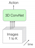
The video frames can be passed in several ways:
(1) In a large batch directly, such as in the first figure. Since we are passing a sequence of frames, both spatial and temporal information is available

(2) We could also pass a single image frame in one stream (spatial information of the data) and its corresponding optical flow representation from the video (temporal information of the data). We’ll extract features from both using regular 2D CNNs, before combining them to be passed to our 3D CNN, which combines both types of information
(3) Pass our sequence of frames to one 3D CNN and the optical flow representation of the video to another 3D CNN. Both of the data streams have spatial and temporal information available. This would be the slowest option but also potentially the most accurate, given that we are doing specific processing for two different representations of our video that both contain all of our information.
All of these networks output the action classification of the video.
Like to learn?
Follow me on twitter where I post all about the latest and greatest AI, Technology, and Science!
Bio: George Seif is a Certified Nerd and AI / Machine Learning Engineer.
Original. Reposted with permission.
Related:
- Solve any Image Classification Problem Quickly and Easily
- An Introduction to Scikit Learn: The Gold Standard of Python Machine Learning
- How to Setup a Python Environment for Machine Learning