Deconstructing BERT: Distilling 6 Patterns from 100 Million Parameters
Google’s BERT algorithm has emerged as a sort of “one model to rule them all.” BERT builds on two key ideas that have been responsible for many of the recent advances in NLP: (1) the transformer architecture and (2) unsupervised pre-training.
By Jesse Vig, Research Scientist
The year 2018 marked a turning point for the field of Natural Language Processing, with a series of deep-learning models achieving state-of-the-art results on NLP tasks ranging from question answering to sentiment classification. Most recently, Google’s BERT algorithm has emerged as a sort of “one model to rule them all,” based on its superior performance over a wide variety of tasks.
BERT builds on two key ideas that have been responsible for many of the recent advances in NLP: (1) the transformer architecture and (2) unsupervised pre-training. The transformer is a sequence model that forgoes the sequential structure of RNN’s for a fully attention-based approach, as described in the classic Attention Is All You Need. BERT is also pre-trained; its weights are learned in advance through two unsupervised tasks: masked language modeling (predicting a missing word given the left and right context) and next sentence prediction (predicting whether one sentence follows another). Thus BERT doesn’t need to be trained from scratch for each new task; rather, its weights are fine-tuned. For more details about BERT, check out the The Illustrated Bert.
BERT is a (multi-headed) beast
Bert is not like traditional attention models that use a flat attention structure over the hidden states of an RNN. Instead, BERT uses multiple layers of attention (12 or 24 depending on the model), and also incorporates multiple attention “heads” in every layer (12 or 16). Since model weights are not shared between layers, a single BERT model effectively has up to 24 x 16 = 384 different attention mechanisms.
Visualizing BERT
Because of BERT’s complexity, it can be difficult to intuit the meaning of its learned weights. Deep-learning models in general are notoriously opaque, and various visualization tools have been developed to help make sense of them.
However, I hadn’t found one that could shed light on the attention patterns that BERT was learning. Fortunately, Tensor2Tensor has an excellent tool for visualizing attention in encoder-decoder transformer models, so I modified this to work with BERT’s architecture, using a PyTorch implementation of BERT. The adapted interface is shown below. You can run it directly in this Colab notebook, or find it on Github,
The tool visualizes attention as lines connecting the position being updated (left) with the position being attended to (right). Colors identify the corresponding attention head(s), while line thickness reflects the attention score. At the top of the tool, the user can select the model layer, as well as one or more attention heads (by clicking on the color patches at the top, representing the 12 heads).
What does BERT actually learn?
I used the tool to explore the attention patterns of various layers / heads of the pre-trained BERT model (the BERT-Base, uncased version). I experimented with different input values, but for demonstration purposes, I just use the following inputs:
Sentence A: I went to the store.
Sentence B: At the store, I bought fresh strawberries.
BERT uses WordPiece tokenization and inserts special classifier ([CLS]) and separator ([SEP]) tokens, so the actual input sequence is: [CLS] i went to the store . [SEP] at the store , i bought fresh straw ##berries . [SEP]
I found some fairly distinctive and surprisingly intuitive attention patterns. Below I identify six key patterns and for each one I show visualizations for a particular layer / head that exhibited the pattern.
Pattern 1: Attention to next word
In this pattern, most of the attention at a particular position is directed to the next token in the sequence. Below we see an example of this for layer 2, head 0. (The selected head is indicated by the highlighted square in the color bar at the top.) The figure on the left shows the attention for all tokens, while the one on the right shows the attention for one selected token (“i”). In this example, virtually all of the attention is directed to “went,” the next token in the sequence.
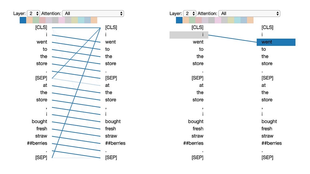
On the left, we can see that the [SEP] token disrupts the next-token attention pattern, as most of the attention from [SEP] is directed to [CLS] rather than the next token. Thus this pattern appears to operate primarily within each sentence.
This pattern is related to the backward RNN, where state updates are made sequentially from right to left. Pattern 1 appears over multiple layers of the model, in some sense emulating the recurrent updates of an RNN.
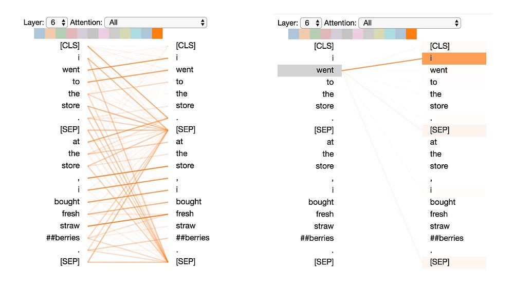
Pattern 2: Attention to previous word
In this pattern, much of the attention is directed to the previous token in the sentence. For example, most of the attention for “went” is directed to the previous word “i” in the figure below. The pattern is not as distinct as the last one; some attention is also dispersed to other tokens, especially the [SEP]tokens. Like Pattern 1, this is loosely related to a sequential RNN, in this case the forward RNN.
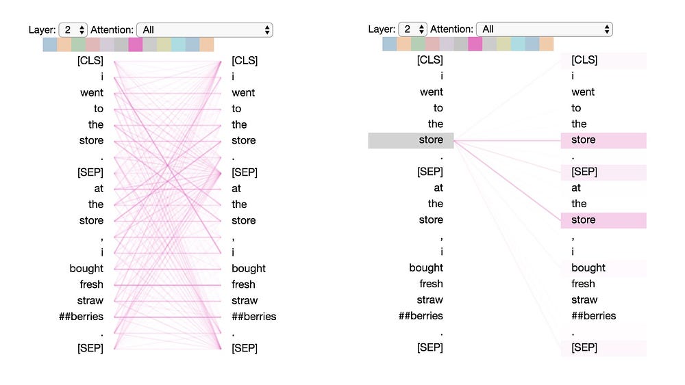
Pattern 3: Attention to identical/related words
In this pattern, attention is paid to identical or related words, including the source word itself. In the example below, most of the attention for the first occurrence of “store” is directed to itself and to the second occurrence of “store”. This pattern is not as distinct as some of the others, with attention dispersed over many different words.
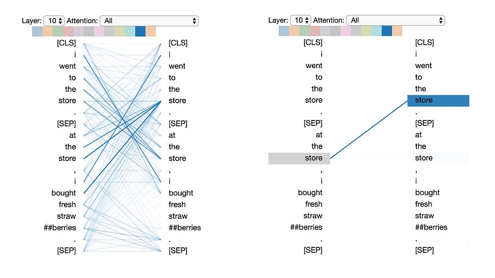
Pattern 4: Attention to identical/related words in other sentence
In this pattern, attention is paid to identical or related words in the other sentence. For example, most of attention for “store” in the second sentence is directed to “store” in the first sentence. One can imagine this being particularly helpful for the next sentence prediction task (part of BERT’s pre-training), because it helps identify relationships between sentences.
Pattern 5: Attention to other words predictive of word
In this pattern, attention seems to be directed to other words that are predictive of the source word, excluding the source word itself. In the example below, most of the attention from “straw” is directed to “##berries”, and most of the attention from “##berries” is focused on “straw”.
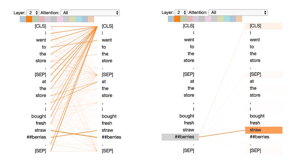
This pattern isn’t as distinct as some of the others. For example, much of the attention is directed to a delimiter token ([CLS]), which is the defining characteristic of Pattern 6 discussed next.
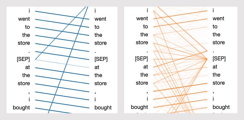
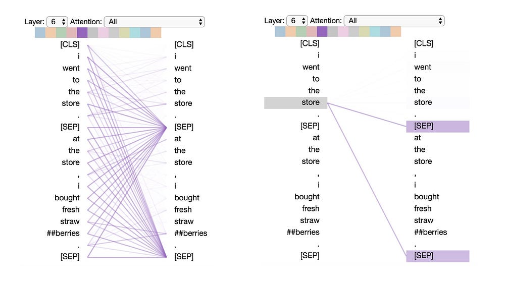
Pattern 6: Attention to delimiter tokens
In this pattern, most of the attention is directed to the delimiter tokens, either the [CLS] token or the [SEP] tokens. In the example below, most of the attention is directed to the two [SEP] tokens. This may be a way for the model to propagate sentence-level state to the individual tokens.
Notes
It has been said that data visualizations are a bit like Rorschach tests: our interpretations may be colored by our own beliefs and expectations. While some of the patterns above are quite distinct, others are somewhat subjective, so these interpretations should only be taken as preliminary observations.
Also, the above 6 patterns describe the coarse attentional structure of BERT and do not attempt to describe the linguistic patterns that attention may capture. For example, there are many different types of “relatedness” that could manifest in Patterns 3 and 4, e.g., synonymy, coreference, etc. It would be interesting to see if different attention heads specialize in different types of semantic and syntactic relationships.
Try it out!
As mentioned earlier, you can run the BERT visualizer directly in this Colab Notebook. (If you scroll to the bottom of the notebook, you may be able to use the tool without running the code). You can also check out the Github repo. Please play with it and share what you find!
[UPDATE]: In Part 2, I extend the visualization tool to show how BERT is able to form its distinctive attention patterns.
Big thanks to Llion Jones for creating the original Tensor2Tensor visualization tool!
Bio: Jesse Vig is a research scientist working on natural language processing and conversational AI. He also likes to explore the intersection of machine learning and human-computer interaction, particular around data visualization.
Original. Reposted with permission.
Related:
- Are BERT Features InterBERTible?
- 10 Exciting Ideas of 2018 in NLP
- Word Embeddings in NLP and its Applications