Deconstructing BERT, Part 2: Visualizing the Inner Workings of Attention
In this post, the author shows how BERT can mimic a Bag-of-Words model. The visualization tool from Part 1 is extended to probe deeper into the mind of BERT, to expose the neurons that give BERT its shape-shifting superpowers.
By Jesse Vig, Research Scientist
In Deconstructing BERT: Distilling 6 Patterns from 100 Million Parameters, I described how BERT’s attention mechanism can take on many different forms. For example, one attention head focused nearly all of the attention on the next word in the sequence; another focused on the previous word (see illustration below). In both cases, BERT essentially learned a sequential update pattern, something that human designers of neural networks have explicitly encoded in architectures such as Recurrent Neural Networks (though BERT’s version is more like a CNN). Later, I will show how BERT is able to mimic a Bag-of-Words model as well.
So how does BERT achieve these stunning feats of plasticity? To answer this question, I extend the visualization tool from Part 1 to probe deeper into the mind of BERT, to expose the neurons that give BERT its shape-shifting superpowers. You can try the updated visualization tool in this Colab notebook, or find it on Github.
The original visualization tool (based on the excellent Tensor2Tensorimplementation by Llion Jones) attempted to answer the what of attention: that is, what attention structures is BERT learning? To answer the how, I added an attention details view, which visualizes how attention is computed. The details view is invoked by clicking on the ⊕ icon. You can see a demo below, or skip ahead to the screen shots:
Visualization Tool Overview
BERT is a bit like a Rube Goldberg machine: though the individual components are fairly intuitive, the end-to-end system can be hard to grasp. For now, I’ll walk through the parts of BERT’s attention architecture represented in the visualization tool. (For a comprehensive tutorial on BERT, I recommend The Illustrated Transformer and The Illustrated BERT.)
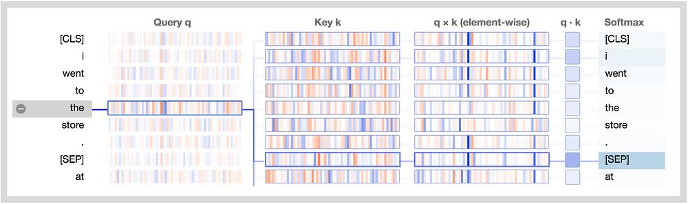
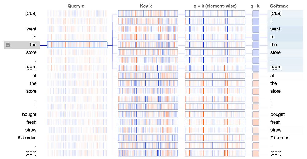
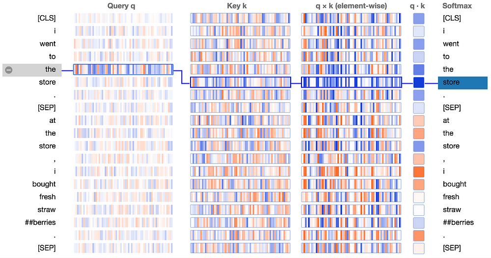
The new attention details view is shown below. Note that positive values are colored blue and negative values orange, with color intensity reflecting the magnitude of the value. All vectors are of length 64 and are specific to a particular attention head. Like the original visualization tool, connecting lines are weighted based on the attention score between the respective words.
Let’s break this down:
Query q: the query vector q encodes the word/position on the left that is paying attention, i.e. the one that is “querying” the other words. In the example above, the query vector for “the” (the selected word) is highlighted.
Key k: the key vector k encodes the word on the right to which attention is being paid. The key vector together with the query vector determine the attention score between the respective words, as described below.
q×k (element-wise): the element-wise product of the query vector and a key vector. This product is computed between the selected query vector and each of the key vectors. This is a precursor to the dot product (the sum of the element-wise product) and is included for visualization purposes because it shows how individual elements in the query and key vectors contribute to the dot product.
q·k: the dot product of the selected query vector and each of the key vectors. This is the unnormalized attention score.
Softmax: the softmax of q·k / 8 across all target words. This normalizes the attention scores to be positive and sum to one. The constant factor 8 is the square root of the vector length (64), and is included for reasons described in this paper.
Explaining BERT’s attention patterns
In Part 1, I identified several patterns in the attention structure across BERT’s attention heads. Let’s see if we can use the visualization tool to understand how BERT forms these patterns.
Delimiter-focused attention patterns
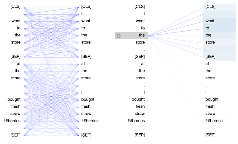
Let’s start with the simple case where most attention is focused on the sentence separator [SEP] token (Pattern 6 from Part 1). As suggested in Part 1, this pattern may be a way for BERT to propagate sentence-level state to the word level:
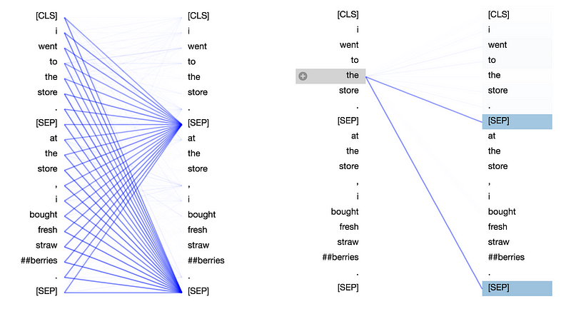
So, how exactly is BERT able to fixate on the [SEP] tokens? Let’s see if the visualization tool can provide some clues. Here we see the attention details view of the example above:
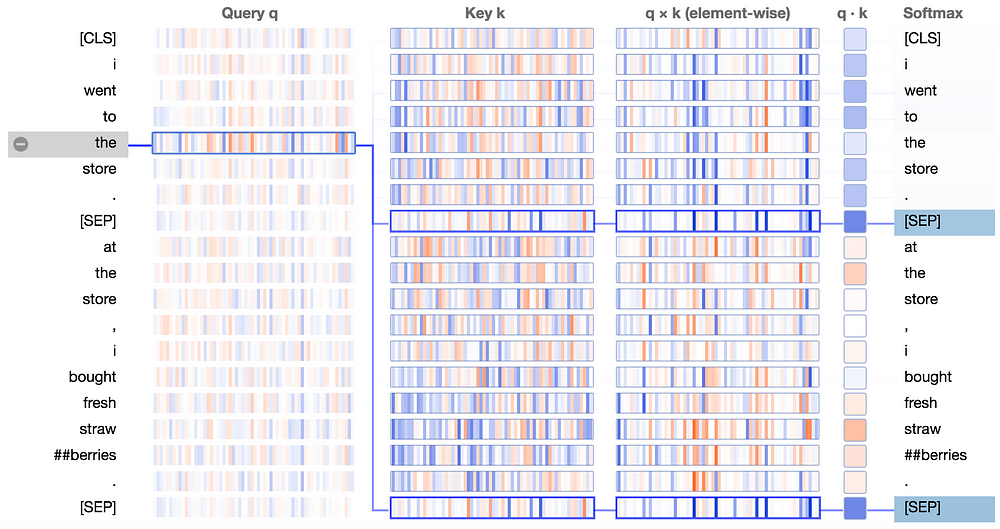
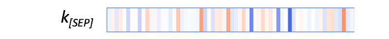
In the Key column, the key vectors for the two occurrences of [SEP] carry a distinctive signature: they both have a small number of active neurons with high positive (blue) or low negative (orange) values, and a larger number of neurons with values close to zero (light blue/orange or white):
The query vectors tend to match the [SEP] key vectors along those active neurons, resulting in high values for the element-wise product q×k, as in this example:
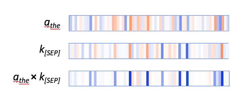
The query vectors for the other words follow a similar pattern: they match the [SEP] key vector along the same set of neurons. Thus it seems that BERT has designated a small set of neurons as “[SEP]-matching neurons,” and query vectors are assigned values that match the [SEP] key vectors at these positions. The result is the [SEP]-focused attention pattern.
Bag of Words attention pattern
This is a less common pattern, which was not discussed in Part 1. In this pattern, attention is divided fairly evenly across all words in the same sentence:
The effect of this pattern is to distribute sentence-level state to the word level, as was likely the case for the first pattern as well. BERT is essentially computing a Bag-of-Words embedding by taking an (almost) unweighted average of the word embeddings (which are the value vectors — see above-mentioned tutorials for details on this.)
So how does BERT finesse the queries and keys to form this attention pattern? Let’s again turn to the attention details view:
In the q×k column, we see a clear pattern: a small number of neurons (2–4) dominate the calculation of the attention scores. When query and key vector are in the same sentence (the first sentence, in this case), the product shows high values (blue) at these neurons. When query and key vector are in different sentences, the product is strongly negative (orange) at these same positions, as in this example:
When query and key are both from sentence 1, they tend to have values with the same sign along the active neurons, resulting in a positive product. When the query is from sentence 1, and the key is from sentence 2, the same neurons tend to have values with opposite signs, resulting in a negative product.
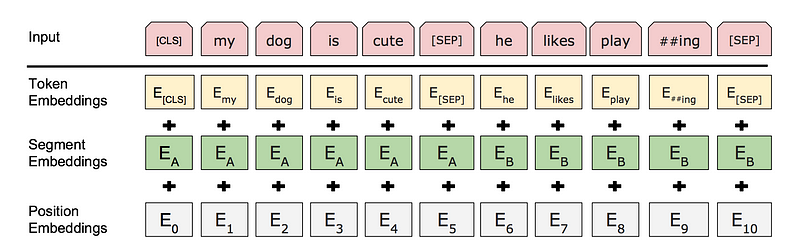
But how does BERT know the concept of “sentence”, especially in the first layer of the network before higher-level abstractions are formed? The answer lies in the sentence-level embeddings that are added to the input layer (see Figure 1, below). The information encoded in these sentence embeddings flows to downstream variables, i.e. queries and keys, and enables them to acquire sentence-specific values.
Next-word attention patterns
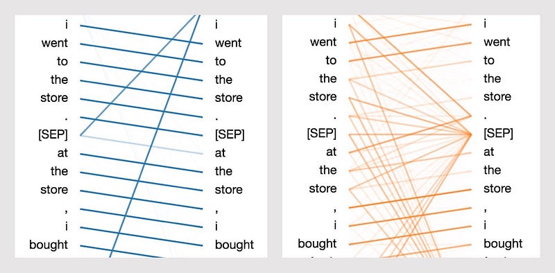
In the next-word attention pattern, virtually all the attention is focused on the next word in the input sequence, except at the delimiter tokens:
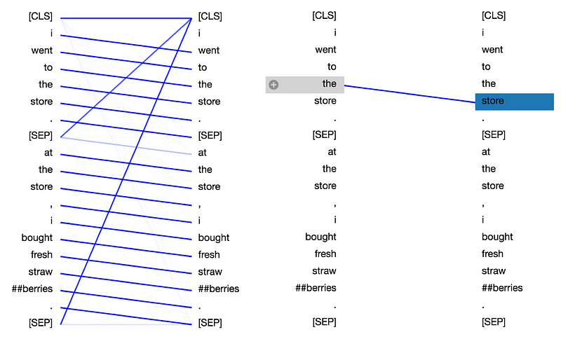
This attention pattern enables BERT to capture sequential relationships, e.g. bigrams. Let’s check out the attention detail view for the above example:
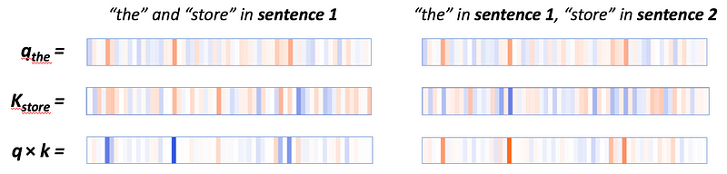
We see that the product of the query vector for “the” and the key vector for “store” (the next word) is strongly positive across most neurons. For tokens other than the next token, the key-query product contains some combination of positive and negative values. The result is a high attention score between “the” and “store”.
For this attention pattern, a large number of neurons figure into the attention score, and these neurons differ depending on the token position, as illustrated here:
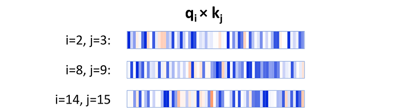
Element-wise product of query and key vectors, for query at position i and key at position j = i+1, for i = 2, 8, 14. Note that the active neurons differ in each case.
This behavior differs from the delimiter-focused and the sentence-focused attention patterns, in which a small, fixed set of neurons determine the attention scores. For those two patterns, only a few neurons are required because the patterns are so simple, and there is little variation in the words that receive attention. In contrast, the next-word attention pattern needs to track which of the 512 words receives attention from a given position, i.e., which is the next word. To do so it needs to generate queries and keys such that each query vector matches with a unique key vector from the 512 possibilities. This would be difficult to accomplish using a small subset of neurons.
So how is BERT able to generate these position-aware queries and keys? In this case, the answer lies in BERT’s position embeddings, which are added to the word embeddings at the input layer (see Figure 1). BERT learns a unique position embedding for each of the 512 positions in the input sequence, and this position-specific information can flow through the model to the key and query vectors.
Notes
I have only covered some of the coarse-level attention patterns discussed in Part 1 and have not touched on lower-level dynamics around linguistic phenomena such as coreference, synonymy, etc. I hope that this tool can help provide intuition in many of these cases.
Try it out!
Please try out the visualization tool and share what you find!
Colab: https://colab.research.google.com/drive/1Nlhh2vwlQdKleNMqpmLDBsAwrv_7NnrB
Github: https://github.com/jessevig/bertviz
Bio: Jesse Vig is a research scientist working on natural language processing and conversational AI. He also likes to explore the intersection of machine learning and human-computer interaction, particular around data visualization.
Original. Reposted with permission.
Related:
- Deconstructing BERT: Distilling 6 Patterns from 100 Million Parameters
- BERT: State of the Art NLP Model, Explained
- Are BERT Features InterBERTible?