Feature Reduction using Genetic Algorithm with Python
This tutorial discusses how to use the genetic algorithm (GA) for reducing the feature vector extracted from the Fruits360 dataset in Python mainly using NumPy and Sklearn.

Introduction
Using the raw data for training a machine learning algorithm might not be the suitable choice in some situations. The algorithm, when trained by raw data, has to do feature mining by itself for detecting the different groups from each other. But this requires large amounts of data for doing feature mining automatically. For small datasets, it is preferred that the data scientist do the feature mining step on its own and just tell the machine learning algorithm which feature set to use.
The used feature set has to be representative of the data samples and thus we have to take care of selecting the best features. The data scientist suggests using some types of features that seems helpful in representing the data samples based on the previous experience. Some features might prove their robustness in representing the samples and others not.
There might be some types of feature that might affect the results of the trained model wither by reducing the accuracy for classification problems or increasing the error for regression problems. For example, there might be some noise elements in the feature vector and thus they should get removed. The feature vector might also include 2 or more correlated elements. Just using one element will substitute for the other. In order to remove such types of elements, there are 2 helpful steps which are feature selection and reduction. This tutorial focuses on feature reduction.
Assuming there are 3 features F1, F2, and F3 and each one has 3 feature elements. Thus, the feature vector length is 3x3=9. Feature selection just selects specific types of features and excludes the others. For example, just select F1 and F3 and remove F3. The feature vector length is now 6 rather than 9. In feature reduction, specific elements from each feature might be excluded. For example, this step might remove the first and third elements from F3 while keeping the second element. Thus, the feature vector length is reduced from 9 to just 7.
Before starting in this tutorial, it is worth mentioning that it is an extension to a previously published 2 tutorials in my LinkedIn profile.
The first tutorial is titled "Artificial Neural Network Implementation using NumPy and Classification of the Fruits360 Image Dataset". It starts by extracting a feature vector of length 360 from 4 classes of the Fruits360 dataset. Then, it builds an artificial neural network (ANN) using NumPy from scratch in order to classify the dataset. It is available here https://www.linkedin.com/pulse/artificial-neural-network-implementation-using-numpy-fruits360-gad. Its GitHub project is available here: https://github.com/ahmedfgad/NumPyANN.
The second tutorial is titled "Artificial Neural Networks Optimization using Genetic Algorithm". It builds and uses the GA for optimizing the ANN parameters in order to increase the classification accuracy. It is available here https://www.linkedin.com/pulse/artificial-neural-networks-optimization-using-genetic-ahmed-gad. Its GitHub project is also available here: https://github.com/ahmedfgad/NeuralGenetic.
This tutorial discusses how to use the genetic algorithm (GA) for reducing the feature vector extracted from the Fruits360 dataset of length 360. This tutorial starts by discussing the steps to be followed. After that, the steps are implemented in Python mainly using NumPy and Sklearn.
The implementation of this tutorial is available in my GitHub page here: https://github.com/ahmedfgad/FeatureReductionGenetic
GA starts from an initial population which consists of a number of chromosomes (i.e. solutions) where each chromosome has a sequence of genes. Using a fitness function, the GA selects the best solutions as parents for creating a new population. The new solutions in such a new population are created by applying 2 operations over the parents which are the crossover and the mutation. When applying GA to a given problem, we have to determine the representation of the gene, the suitable fitness function, and how the crossover and the mutation are applied. Let’s see how things work.
More Information about GA
You can read more about GA from the following resources I prepared:
- Introduction to Optimization with Genetic Algorithm
- Genetic Algorithm (GA) Optimization - Step-by-Step Example
- Genetic Algorithm Implementation in Python
I also wrote a book in 2018 that covers GA in one of its chapters. The book is titled "Practical Computer Vision Applications Using Deep Learning with CNNs" which is available here at Springer https://www.springer.com/us/book/9781484241660.
Chromosome Representation
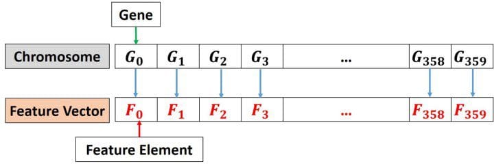
The gene in GA is the building block for the chromosome. At first, we need to determine what genes are inside the chromosome. To do that, take into regard that every property that may affect the results should be regarded as a gene. Because the target of our problem is selecting the best set of feature elements, thus every feature element might affect the results if selected or not. Thus, every feature element is regarded as a gene. The chromosome will consist of all genes (i.e. all feature elements). Because there are 360 feature elements, then there will be 360 genes. A good piece of information is now clear that the length of the chromosome is 360.
After determining what are the selected genes, next is to determine the gene representation. There are different representations such as decimal, binary, float, string, and others. Our target is to know whether the gene (i.e. feature element) is selected or not in the reduced set of features. Thus, the value assigned to the gene should reflect whether it is selected or not. Based on this description, it is very clear that there are 2 possible values for each gene. One value signifies that the gene is selected and another when it is not selected. Thus, the binary representation is the best choice. When the gene value is 1, then it will be selected in the reduced feature set. When 0, then it will be neglected.
As a summary, the chromosome will consist of 360 genes represented in binary. There is a one-to-one mapping between the feature vector and the chromosome according to the next figure. That is the first gene in the chromosome is linked to the first element in the feature vector. When the value for that gene is 1, this means the first element in the feature vector is selected.
Fitness Function
By getting how to create the chromosome, the initial population can be initialized randomly easily is NumPy. After being initialized, the parents are selected. GA is based on Darwin’s theory "Survival of the Fittest". That is the best solutions in the current population are selected for mating in order to produce better solutions. By keeping the good solutions and killing the bad solutions, we can reach an optimal or semi-optimal solution.
The criterion used for selecting the parents is the fitness value associated with each solution (i.e. chromosome). The higher the fitness value the better the solution. The fitness value is calculated using a fitness function. So, what is the best function for use in our problem? The target of our problem is creating a reduced feature vector that increases the classification accuracy. Thus, the criterion that judges whether a solution is good or not is the classification accuracy. As a result, the fitness function will return a number that specifies the classification accuracy for each solution. The higher the accuracy the better the solution.
In order to return a classification accuracy, there must be a machine learning model to get trained by the feature elements returned by each solution. We will use the support vector classifier (SVC) for this case.
The dataset is divided into train and test samples. Based on the train data, the SVC will be trained using the selected feature elements by each solution in the population. After being trained, it will be tested according to the test data.
Based on the fitness value of each solution, we can select the best of them as parents. These parents are placed together in the mating pool for generating offspring which will be the members of the new population of the next generation. Such offspring are created by applying the crossover and mutation operations over the selected parents. Let’s configure such operations as discussed next.
Crossover and Mutation
Based on the fitness function, we can filter the solutions in the current population for selecting the best of them which are called the parents. GA assumes that mating 2 good solutions will produce a third better solution. Mating means exchanging some genes from 2 parents. The genes are exchanged using the crossover operation. There are different ways in which such an operation can be applied. This tutorial uses the single-point crossover in which a point divides the chromosome. Genes before the point are taken from one solution and genes after the point are taken from the other solution.
By just applying crossover, all genes are taken from the previous parents. There is no new gene introduced in the new offspring. If there is a bad gene in all parents, then this gene will be transferred to the offspring. For such a reason, the mutation operation is applied in order to introduce new genes in the offspring. In the binary representation of the genes, the mutation is applied by flipping the values of some randomly selected genes. If the gene value is 1, then it will be 0 and vice versa.
After generating the offspring, we can create the new population of the next generation. This population consists of the previous parents in addition to the offspring.
At this point, all steps are discussed. Next is to implement them in Python. Note that I wrote a previous tutorial titled "Genetic Algorithm Implementation in Python" for implementing the GA in Python which I will just modify its code for working with our problem. It is better to read it.
Python Implementation
The project is organized into 2 files. One file is named "GA.py" which holds the implementation of the GA steps as functions. Another file, which is the main file, just imports this file and calls its function within a loop that iterates through the generations.
The main file starts by reading the features extracted from the Fruits360 dataset according to the code below. The features are returned into the data_inputs variable. Details about extracting these features are available in the 2 tutorials referred to at the beginning of the tutorial. The file also reads the class labels associated with the samples in the variable data_outputs.
Some samples are selected for training with their indices stored in the train_indices variable. Similarly, the test samples indices are stored in the test_indices variable.
import numpy

import GA

import pickle

import matplotlib.pyplot


f = open("dataset_features.pkl", "rb")

data_inputs = pickle.load(f)

f.close()


f = open("outputs.pkl", "rb")

data_outputs = pickle.load(f)

f.close()


num_samples = data_inputs.shape[0]

num_feature_elements = data_inputs.shape[1]


train_indices = numpy.arange(1, num_samples, 4)

test_indices = numpy.arange(0, num_samples, 4)

print("Number of training samples: ", train_indices.shape[0])

print("Number of test samples: ", test_indices.shape[0])


"""

Genetic algorithm parameters:

    Population size

    Mating pool size

    Number of mutations
"""

sol_per_pop = 8 # Population size.

num_parents_mating = 4 # Number of parents inside the mating pool.

num_mutations = 3 # Number of elements to mutate.

# Defining the population shape.
pop_shape = (sol_per_pop, num_feature_elements)

# Creating the initial population.
new_population = numpy.random.randint(low=0, high=2, size=pop_shape)
print(new_population.shape)

best_outputs = []
num_generations = 100
It initializes all parameters of GA. This includes the number of solutions per population which is set to 8 according to the sol_per_pop variable, number of offspring which is set to 4 in the num_parents_mating variable, and number of mutations which is set to 3 in the num_mutations variable. After that, it creates the initial population randomly in a variable called new_population.
There is an empty list named best_outputs which holds the best result after each generation. This helps to visualize the progress of the GA after finishing all generations. The number of generations is set to 100 in the num_generations variable. Note that you can change all of these parameters which might give better results.