10 Simple Hacks to Speed up Your Data Analysis in Python
This article lists some curated tips for working with Python and Jupyter Notebooks, covering topics such as easily profiling data, formatting code and output, debugging, and more. Hopefully you can find something useful within.
By Parul Pandey, Data Science Enthusiast

Tips and Tricks, especially in the programming world, can be very useful. Sometimes a little hack can be both time and life-saving. A minor shortcut or add-on can sometimes prove to be a Godsend and can be a real productivity booster. So, here are some of my favourite tips and tricks that I have used and compiled together in the form of this article. Some may be fairly known and some may be new but I am sure they would come in pretty handy the next time you work on a Data Analysis project.
1. Profiling the pandas dataframe
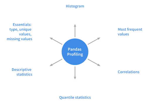
Profiling is a process that helps us in understanding our data and Pandas Profiling is python package which does exactly that. It is a simple and fast way to perform exploratory data analysis of a Pandas Dataframe. The pandas df.describe()and df.info()functions are normally used as a first step in the EDA process. However, it only gives a very basic overview of the data and doesn’t help much in the case of large data sets. The Pandas Profiling function, on the other hand, extends the pandas DataFrame with df.profile_report() for quick data analysis. It displays a lot of information with a single line of code and that too in an interactive HTML report.
For a given dataset the pandas profiling package computes the following statistics:
Installation
pip install pandas-profiling
or
conda install -c anaconda pandas-profiling
Usage
Let’s use the age-old titanic dataset to demonstrate the capabilities of the versatile python profiler.
#importing the necessary packages
import pandas as pd
import pandas_profiling

# Depreciated: pre 2.0.0 version
df = pd.read_csv('titanic/train.csv')
pandas_profiling.ProfileReport(df)
Edit: A week after this article was published, Pandas-Profiling came out with a major upgrade -version 2.0.0. The syntax has changed a bit, in fact, the functionality has been included in the pandas itself and the report has become more comprehensive. Below is the latest usage syntax:
Usage
To display the report in a Jupyter notebook, run:
#Pandas-Profiling 2.0.0
df.profile_report()
This single line of code is all that you need to display the data profiling report in a Jupyter notebook. The report is pretty detailed including charts wherever necessary.
The report can also be exported into an interactive HTML file with the following code.
profile = df.profile_report(title='Pandas Profiling Report')
profile.to_file(outputfile="Titanic data profiling.html")
Refer to the documentation for more details and examples.
2. Bringing Interactivity to pandas plots
Pandas has a built-in .plot() function as part of the DataFrame class. However, the visualisations rendered with this function aren't interactive and that makes it less appealing. On the contrary, the ease to plot charts with pandas.DataFrame.plot() function also cannot be ruled out. What if we could plot interactive plotly like charts with pandas without having to make major modifications to the code? Well, you can actually do that with the help of Cufflinks library.
Cufflinks library binds the power of plotly with the flexibility of pandas for easy plotting. Let’s now see how we can install the library and get it working in pandas.
Installation
pip install plotly # Plotly is a pre-requisite before installing cufflinks
pip install cufflinks
Usage
#importing Pandas
import pandas as pd
#importing plotly and cufflinks in offline mode
import cufflinks as cf

import plotly.offline
cf.go_offline()
cf.set_config_file(offline=False, world_readable=True)
Time to see the magic unfold with the Titanic dataset.
df.iplot()
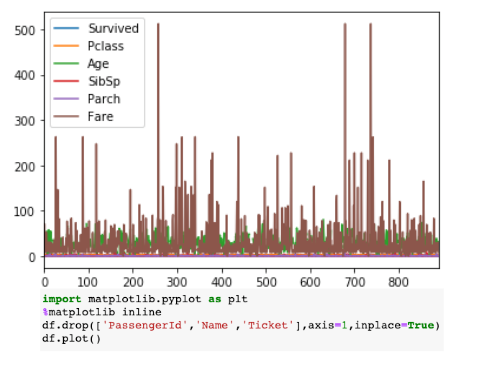
df.iplot() vs df.plot()
The visualisation on the right shows the static chart while the left chart is interactive and more detailed and all this without any major change in the syntax.
Click here for more examples.
3. A Dash of Magic
Magic commands are a set of convenient functions in Jupyter Notebooks that are designed to solve some of the common problems in standard data analysis. You can see all available magics with the help of %lsmagic.
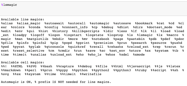
Magic commands are of two kinds: line magics, which are prefixed by a single % character and operate on a single line of input, and cell magics, which are associated with the double %% prefix and operate on multiple lines of input. Magic functions are callable without having to type the initial % if set to 1.
Let’s look at some of them that might be useful in common data analysis tasks:
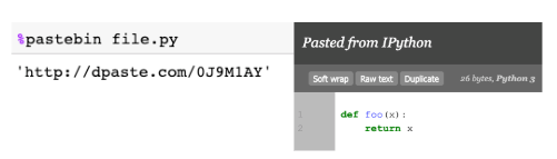
- % pastebin
%pastebin uploads code to Pastebin and returns the url. Pastebin is an online content hosting service where we can store plain text like source code snippets and then the url can be shared with others. In fact, Github gist is also akin to pastebin albeit with version control.
Consider a python script file.py with the following content:
#file.py
def foo(x):
    return x
Using %pastebin in Jupyter Notebook generates a pastebin url.
- %matplotlib notebook
The %matplotlib inline function is used to render the static matplotlib plots within the Jupyter notebook. Try replacing the inline part with notebook to get zoom-able & resize-able plots, easily. Make sure the function is called before importing the matplotlib library.
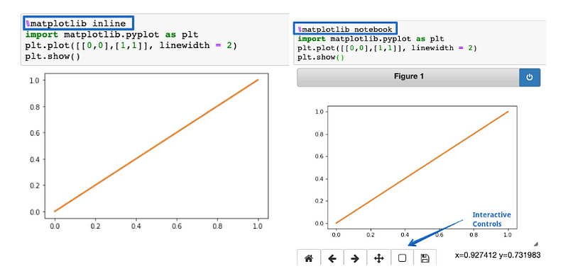
%matplotlib inline vs %matplotlib notebook
- %run
The %run function runs a python script inside a notebook.
%run file.py
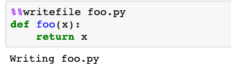
- %%writefile
%%writefile writes the contents of a cell to a file. Here the code will be written to a file named foo.py and saved in the current directory.
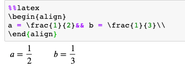
- %%latex
The %%latex function renders the cell contents as LaTeX. It is useful for writing mathematical formulae and equations in a cell.
4. Finding and Eliminating Errors
The interactive debugger is also a magic function but I have given it a category of its own. If you get an exception while running the code cell, type %debug in a new line and run it. This opens an interactive debugging environment which brings you to the position where the exception has occurred. You can also check for values of variables assigned in the program and also perform operations here. To exit the debugger hit q.
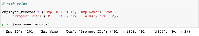
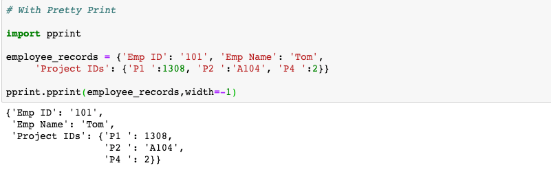
5. Printing can be pretty too
If you want to produce aesthetically pleasing representations of your data structures, pprint is the go-to module. It is especially useful when printing dictionaries or JSON data. Let’s have a look at an example which uses both print and pprint to display the output.
6. Making the Notes stand out.
We can use alert/Note boxes in your Jupyter Notebooks to highlight something important or anything that needs to stand out. The colour of the note depends upon the type of alert that is specified. Just add any or all of the following codes in a cell that needs to be highlighted.
- Blue Alert Box: info
<div class="alert alert-block alert-info">
<b>Tip:</b> Use blue boxes (alert-info) for tips and notes.
If it’s a note, you don’t have to include the word “Note”.
</div>

- Yellow Alert Box: Warning
<div class="alert alert-block alert-warning">
<b>Example:</b> Yellow Boxes are generally used to include additional examples or mathematical formulas.
</div>

- Green Alert Box: Success
<div class="alert alert-block alert-success">
Use green box only when necessary like to display links to related content.
</div>

- Red Alert Box: Danger
<div class="alert alert-block alert-danger">
It is good to avoid red boxes but can be used to alert users to not delete some important part of code etc.
</div>

7. Printing all the outputs of a cell
Consider a cell of Jupyter Notebook containing the following lines of code:
In  [1]: 10+5
         11+6
Out [1]: 17
It is a normal property of the cell that only the last output gets printed and for the others, we need to add the print() function. Well, it turns out that we can print all the outputs just by adding the following snippet at the top of the notebook.
from IPython.core.interactiveshell import InteractiveShell InteractiveShell.ast_node_interactivity = "all"
Now all the outputs get printed one after the other.
In  [1]: 10+5
         11+6
         12+7
Out [1]: 15
Out [1]: 17
Out [1]: 19
To revert to the original setting :
InteractiveShell.ast_node_interactivity = "last_expr"
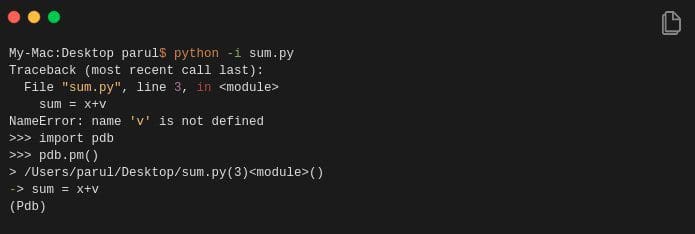
8. Running python scripts with the ‘i’ option.
A typical way of running a python script from the command line is: python hello.py. However, if you add an additional -i while running the same script e.g python -i hello.py it offers more advantages. Let’s see how.
- Firstly, once the end of the program is reached, python doesn’t exit the interpreter. As such we can check the values of the variables and the correctness of the functions defined in our program.

- Secondly, we can easily invoke a python debugger since we are still in the interpreter by:
import pdb
pdb.pm()
This will bring us o the position where the exception has occurred and we can then work upon the code.
The original source of the hack.
9. Commenting out code automatically
Ctrl/Cmd + / comments out selected lines in the cell by automatically. Hitting the combination again will uncomment the same line of code.
10. To delete is human, to restore divine
Have you ever accidentally deleted a cell in a Jupyter Notebook? If yes then here is a shortcut which can undo that delete action.
- In case you have deleted the contents of a cell, you can easily recover it by hitting
CTRL/CMD+Z - If you need to recover an entire deleted cell hit
ESC+ZorEDIT > Undo Delete Cells
Conclusion
In this article, I’ve listed the main tips I have gathered while working with Python and Jupyter Notebooks. I am sure they will be of use to you and you will take back something from this article. Till then Happy Coding!.
Bio: Parul Pandey is a Data Science enthusiast who frequently writes for Data Science publications such as Towards Data Science.
Original. Reposted with permission.
Related:
- Using the ‘What-If Tool’ to investigate Machine Learning models
- Animations with Matplotlib
- PyViz: Simplifying the Data Visualisation Process in Python