XGBoost and Random Forest® with Bayesian Optimisation
This article will explain how to use XGBoost and Random Forest with Bayesian Optimisation, and will discuss the main pros and cons of these methods.
By Edwin Lisowski, CTO at Addepto
Instead of only comparing XGBoost and Random Forest in this post we will try to explain how to use those two very popular approaches with Bayesian Optimisation and that are those models main pros and cons. XGBoost (XGB) and Random Forest (RF) both are ensemble learning methods and predict (classification or regression) by combining the outputs from individual decision trees (we assume tree-based XGB or RF).
Let’s dive deeper into comparison – XGBoost vs Random Forest
XGBoost or Gradient Boosting
XGBoost build decision tree one each time. Each new tree corrects errors which were made by previously trained decision tree.
Example of XGBoost application
At Addepto we use XGBoost models to solve anomaly detection problems e.g. in supervised learning approach. In this case XGB is very helpful because data sets are often highly imbalanced. Examples of such data sets are user/consumer transactions, energy consumption or user behaviour in mobile app.
Pros
Since boosted trees are derived by optimizing an objective function, basically XGB can be used to solve almost all objective function that we can write gradient out. This including things like ranking and poisson regression, which RF is harder to achieve.
Cons
XGB model is more sensitive to overfitting if the data is noisy. Training generally takes longer because of the fact that trees are built sequentially. GBMs are harder to tune than RF. There are typically three parameters: number of trees, depth of trees and learning rate, and the each tree built is generally shallow.
Random Forest
Random Forest (RF) trains each tree independently, using a random sample of the data. This randomness helps to make the model more robust than a single decision tree. Thanks to that RF is less likely to overfit on the training data.
Example of Random Forest application
The random forest dissimilarity has been used in a variety of applications, e.g. to find clusters of patients based on tissue marker data.[1] Random Forest model is very attractive for this kind of applications in the following two cases:
Our goal is to have high predictive accuracy for a high-dimensional problem with strongly correlated features.
Our data set is very noisy and contains a lot of missing values e.g., some of the attributes are categorical or semi-continuous.
Pros
The model tuning in Random Forest is much easier than in case of XGBoost. In RF we have two main parameters: number of features to be selected at each node and number of decision trees. RF are harder to overfit than XGB.
Cons
The main limitation of the Random Forest algorithm is that a large number of trees can make the algorithm slow for real-time prediction. For data including categorical variables with different number of levels, random forests are biased in favor of those attributes with more levels.
Bayesian optimization is a technique to optimise function that is expensive to evaluate.[2] It builds posterior distribution for the objective function and calculate the uncertainty in that distribution using Gaussian process regression, and then uses an acquisition function to decide where to sample. Bayesian optimization focuses on solving the problem:
maxx∈A f(x)
The dimension of hyperparameters (x∈Rd) is often d < 20 in most successful applications.
Typically set A i a hyper-rectangle (x∈Rd:ai ≤ xi ≤ bi). The objective function is continuous which is required to model using Gaussian process regression. It also lacks special structure like concavity or linearity which make futile using techniques that leverage such structure to improve efficiency. Bayesian optimization consists of two main components: a Bayesian statistical model for modeling the objective function and an acquisition function for deciding where to sample next.
After evaluating the objective according to an initial space-filling experimental design they are used iteratively to allocate the remainder of a budget of N evaluations, as shown below:
- Observe at initial points
- While n ≤ N do
Update the posterior probability distribution using all available data
Let xn be a maximizer of the acquisition function
Observe yn = f(xn)
Increment n
end while - Return a solution: the point evaluated with the largest
We can summarize this problem by saying that Bayesian optimization is designed for black-box derivative-free global optimization. It has become extremely popular for tuning hyperparameters in machine learning.
Below is a graphical summary of the whole optimization: Gaussian Process with posterior distribution along with observations and confidence interval, and Utility Function where the maximum value indicates the next sample point.
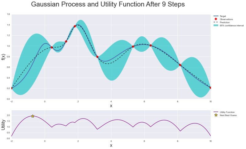
Thanks to utility function bayesian optimization is much more efficient in tuning parameters of machine learning algorithms than grid or random search techniques. It can effectively balance “exploration” and “exploitation” in finding global optimum.
To present Bayesian optimization in action we use BayesianOptimization [3] library written in Python to tune hyperparameters of Random Forest and XGBoost classification algorithms. We need to install it via pip:
pip install bayesian-optimization
Now let’s train our model. First we import required libraries:
#Import libraries
import pandas as pd
import numpy as np
from bayes_opt import BayesianOptimization
from sklearn.ensemble import RandomForestClassifier
from sklearn.model_selection import cross_val_score
We define a function to run Bayesian optimization given data, function to optimize and its hyperparameters:
#Bayesian optimization
def bayesian_optimization(dataset, function, parameters):
   X_train, y_train, X_test, y_test = dataset
   n_iterations = 5
   gp_params = {"alpha": 1e-4}

   BO = BayesianOptimization(function, parameters)
   BO.maximize(n_iter=n_iterations, **gp_params)

   return BO.max
We define function to optimize which is Random Forest Classifier and its hyperparameters n_estimators, max_depth and min_samples_split. Additionally we use the mean of cross validation score on given dataset:
def rfc_optimization(cv_splits):
    def function(n_estimators, max_depth, min_samples_split):
        return cross_val_score(
               RandomForestClassifier(
                   n_estimators=int(max(n_estimators,0)),
                   max_depth=int(max(max_depth,1)),
                   min_samples_split=int(max(min_samples_split,2)),
                   n_jobs=-1,
                   random_state=42,
                   class_weight="balanced"),
               X=X_train,
               y=y_train,
               cv=cv_splits,
               scoring="roc_auc",
               n_jobs=-1).mean()

    parameters = {"n_estimators": (10, 1000),
                  "max_depth": (1, 150),
                  "min_samples_split": (2, 10)}

    return function, parameters
Analogically we define a function and hyperparameters for XGBoost classifier:
def xgb_optimization(cv_splits, eval_set):
    def function(eta, gamma, max_depth):
            return cross_val_score(
                   xgb.XGBClassifier(
                       objective="binary:logistic",
                       learning_rate=max(eta, 0),
                       gamma=max(gamma, 0),
                       max_depth=int(max_depth),
                       seed=42,
                       nthread=-1,
                       scale_pos_weight = len(y_train[y_train == 0])/
                                          len(y_train[y_train == 1])),
                   X=X_train,
                   y=y_train,
                   cv=cv_splits,
                   scoring="roc_auc",
                   fit_params={
                        "early_stopping_rounds": 10,
                        "eval_metric": "auc",
                        "eval_set": eval_set},
                   n_jobs=-1).mean()

    parameters = {"eta": (0.001, 0.4),
                  "gamma": (0, 20),
                  "max_depth": (1, 2000)}

    return function, parameters
Now based on chosen classifier we can optimize it and train the model:
#Train model
def train(X_train, y_train, X_test, y_test, function, parameters):
    dataset = (X_train, y_train, X_test, y_test)
    cv_splits = 4

    best_solution = bayesian_optimization(dataset, function, parameters)
    params = best_solution["params"]

    model = RandomForestClassifier(
             n_estimators=int(max(params["n_estimators"], 0)),
             max_depth=int(max(params["max_depth"], 1)),
             min_samples_split=int(max(params["min_samples_split"], 2)),
             n_jobs=-1,
             random_state=42,
             class_weight="balanced")

    model.fit(X_train, y_train)

    return model
As an example data we use a view [dbo].[vTargetMail] from AdventureWorksDW2017 SQL Server database where based on personal data we need to predict whether person buy a bike. As a result of Bayesian optimization we present consecutive function sampling:
| iter | AUC | max_depth | min_samples_split | n_estimators |
| 1 | 0.8549 | 45.88 | 6.099 | 34.82 |
| 2 | 0.8606 | 15.85 | 2.217 | 114.3 |
| 3 | 0.8612 | 47.42 | 8.694 | 306.0 |
| 4 | 0.8416 | 10.09 | 5.987 | 563.0 |
| 5 | 0.7188 | 4.538 | 7.332 | 766.7 |
| 6 | 0.8436 | 100.0 | 2.0 | 448.6 |
| 7 | 0.6529 | 1.012 | 2.213 | 315.6 |
| 8 | 0.8621 | 100.0 | 10.0 | 1e+03 |
| 9 | 0.8431 | 100.0 | 2.0 | 154.1 |
| 10 | 0.653 | 1.0 | 2.0 | 1e+03 |
| 11 | 0.8621 | 100.0 | 10.0 | 668.3 |
| 12 | 0.8437 | 100.0 | 2.0 | 867.3 |
| 13 | 0.637 | 1.0 | 10.0 | 10.0 |
| 14 | 0.8518 | 100.0 | 10.0 | 10.0 |
| 15 | 0.8435 | 100.0 | 2.0 | 317.6 |
| 16 | 0.8621 | 100.0 | 10.0 | 559.7 |
| 17 | 0.8612 | 89.86 | 10.0 | 82.96 |
| 18 | 0.8616 | 49.89 | 10.0 | 212.0 |
| 19 | 0.8622 | 100.0 | 10.0 | 771.7 |
| 20 | 0.8622 | 38.33 | 10.0 | 469.2 |
| 21 | 0.8621 | 39.43 | 10.0 | 638.6 |
| 22 | 0.8622 | 83.73 | 10.0 | 384.9 |
| 23 | 0.8621 | 100.0 | 10.0 | 936.1 |
| 24 | 0.8428 | 54.2 | 2.259 | 122.4 |
| 25 | 0.8617 | 99.62 | 9.856 | 254.8 |
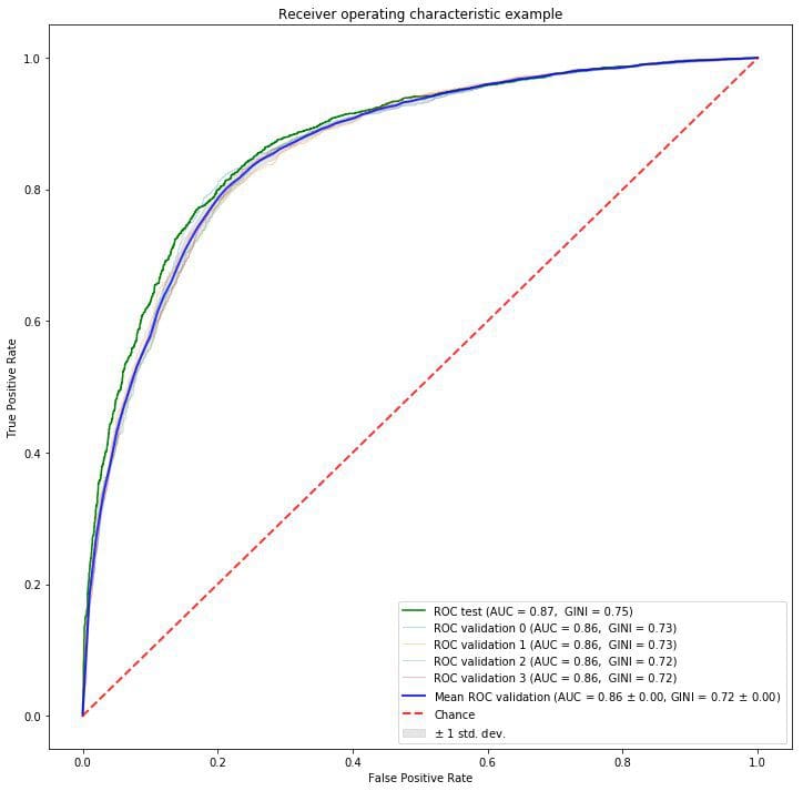
As we can see Bayesian optimization found the best parameters in 23rd step which gives 0.8622 AUC score on test dataset. Probably this result can be higher if given more samples to check. Our optimized Random Forest model has ROC AUC curve presented below:
We presented a simple way of tuning hyperparameters in machine learning [4] using Bayesian optimization which is a faster method in finding optimal values and more sophisticated one than Grid or Random Search methods.
- https://www.researchgate.net/publication/225175169
- https://en.wikipedia.org/wiki/Bayesian_optimization
- https://github.com/fmfn/BayesianOptimization
- https://addepto.com/automated-machine-learning-tasks-can-be-improved/
Bio: Edwin Lisowski is CTO at Addepto. He is an experienced advanced analytics consultant with a demonstrated history of working in the information technology and services industry. He is skilled in Predictive Modeling, Big Data, Cloud Computing and Advanced Analytics.
Related:
- How to Automate Hyperparameter Optimization
- Intro to XGBoost: Predicting Life Expectancy with Supervised Learning
- Random Forests vs Neural Networks: Which is Better, and When?