Many Heads Are Better Than One: The Case For Ensemble Learning
While ensembling techniques are notoriously hard to set up, operate, and explain, with the latest modeling, explainability and monitoring tools, they can produce more accurate and stable predictions. And better predictions can be better for business.
By Jay Budzik, ZestFinance.
“The interests of truth require a diversity of opinions.” —J. S. Mill
Banks and lenders are increasingly turning to AI and machine learning to automate their core functions and make more accurate predictions in credit underwriting and fraud detection. ML practitioners can take advantage of a growing number of modeling algorithms, such as simple decision trees, random forests, gradient boosting machines, deep neural networks, and support vector machines. Each method has its strengths and weaknesses, which is why it often makes sense to combine ML algorithms to provide even greater predictive performance than any single ML method could provide on its own. (This is our standard practice at ZestFinance in every project.) This method of combining algorithms is known as ensembling.
Ensembles improve generalization performance in many scenarios, including classification, regression, and class probability estimation. Ensemble methods have set numerous world records on challenging datasets. An ensemble model won the Netflix Prize and international data science competitions in almost every domain, including predicting credit risk and classifying videos. While ensembles are generally understood to perform better than single-model predictive functions, they are notoriously hard to set up, operate, and explain. These challenges are falling away with the invention of better modeling, explainability and monitoring tools, which we will touch on at the end of this post.
How ensemble models achieve better performance
Just as diversity in nature contributes to more robust biological systems, ensembles of ML models produce stronger results by combining the strengths (and compensating for the weaknesses) of multiple submodels. Neural networks require explicit handling of missing values prior to modeling, but gradient boosted trees handle them automatically. Modelers can introduce bias and errors in the act of making choices about how to handle missing data for neural networks. Error and bias can also enter in from the choices the modeling method makes in the case of gradient boosted trees. Combining different methods (for instance, by averaging or blending the scores) can improve predictions. More specifically, ensembles reduce bias and variance by incorporating different estimators with different patterns of error, diminishing the impact of a single source of error.
There are countless ways to apply ensemble techniques. Submodels can work on different raw input data, and you can even use submodels to generate features for another model to consume. For example, you could train a model on each segment of the data, such as different income levels, and combine the results.
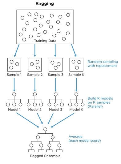
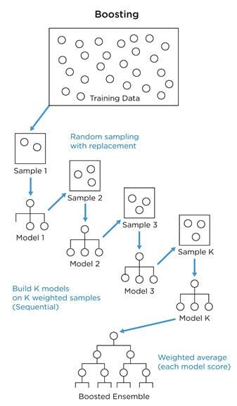
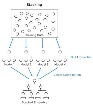
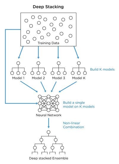
Types of ensembles and how they work
There are four major flavors of ensemble learning:
- In bagging, we use bootstrap sampling to obtain subsets of data for training a set of base models. Bootstrap sampling is the process of using increasingly large random samples until you achieve diminishing returns in predictive accuracy. Each sample is used to train a separate decision tree, and the results of each model are aggregated. For classification tasks, each model votes on an outcome. In regression tasks, the model result is averaged. Base models with low bias but high variance are well-suited for bagging. Random forests, which are bagged combinations of decision trees, are the canonical example of this approach.
- In boosting, we improve performance by concentrating modeling efforts on the data that results in more errors (i.e., focus on the hard stuff). We train a sequence of models where more weight is given to examples that were misclassified by earlier iterations. As with bagging, classification tasks are solved through a weighted majority vote, and regression tasks are solved with a weighted sum to produce the final prediction. Base models with a low variance but high bias are well-adapted for boosting. Gradient boosting is a famous example of this approach.
- In stacking, we create an ensemble function that combines the outputs from multiple base models into a single score. The base-level models are trained based on a complete dataset, and then their outputs are used as input features to train an ensemble function. Usually, the ensemble function is a simple linear combination of the base model scores.
- At ZestFinance, we prefer an even more powerful approach called deep stacking, which uses stacked ensembles with nonlinear ensemble functions that take both model scores as inputs and the input data itself. These are useful in uncovering the deeper relationships between submodels and produce greater accuracy than simple linear stacked ensembles by learning when to apply each submodel based on its strengths. Deep stacking allows the model to select the right submodel weights based on specific input variables (like a product segment, income band, or marketing channel) to boost performance even further.
Results on a real-world credit risk model
To demonstrate the superior performance of ensemble learning, we built a series of binary classification models to predict defaults from a database of auto loans made over three recent years. The loan data included more than 100,000 borrowers and more than 1,100 features.
The competition was between six base machine learning models: four XGBoost models and two neural network models built using features from different sets of credit bureau data, and a combined ensemble model stacking these six base models using a neural network.
To evaluate the accuracy of the models, we measured their AUC and KS scores on the validation data. AUC (area under the receiver operating curve) is used to measure a model’s false positive and false negative rates, while KS (short for Kolmogorov–Smirnov test) is used to compare data distributions. Higher numbers correlate to better business results.
Below are the results of how each model performs in predictive accuracy and dollars saved through lower losses compared to a logistic regression baseline model.
| Model Type | AUC | KS | Est. Dollars Saved |
| Ensemble | 0.803 | 0.446 | $21M |
| XGB 1 | 0.791 (2%) | 0.420 (6%) | $18M (14%) |
| XGB 2 | 0.791 (2%) | 0.428 (4%) | $18M (12%) |
| XGB 3 | 0.781 (3%) | 0.411 (9%) | $17M (16%) |
| XGB 4 | 0.782 (3%) | 0.413 (8%) | $17M (16%) |
| ANN 1 | 0.750 (7%) | 0.376 (19%) | $16M (19%) |
| ANN 2 | 0.786 (2%) | 0.430 (4%) | $18M (13%) |
Our ensemble model produces the highest AUC (0.803), which means that 80% of the time our ensemble ranks a random good applicant more highly than a random bad one. The ensemble’s AUC was 2% better than the best XGBoost and neural network models, which might not sound like much, but AUC is in log scale, so even small increases are more impactful than they appear (similar to the Richter scale for earthquakes). This $500 million-dollar loan business would save $3 million more per year by using the ensemble compared to a single XGBoost or neural network.
The advantages of ensembling extend beyond predictive accuracy. They also benefit the business by improving stability over time. To verify that, using the validation set, we computed the daily AUC score over six months for the ensemble and the submodels on their own. The ensemble model has a 3% lower AUC variance across that time period than the best-performing neural network model and a 21% lower AUC variance than the best-performing XGBoost model. Better stability leads to more predictable results for the business over time.
Challenges with ensembles
We’ve seen above that ensembles produce better economics and better stability in a real-world credit risk modeling problem. However, using complex ensembles in production can be tricky.
Engineering complexity
The we mentioned above? It was too complex for even Netflix to put into production. Technical dependencies, runtime performance, and model verification are all practical challenges associated with using these kinds of models in production. We designed ZAML software tools from the ground up to manage these engineering complexities and we are proud to have many customers with world-class ensembles operating in production.
Producing accurate explanations for the results of ensemble models is particularly challenging. Many explainability methods are model-dependent and do not make problematic assumptions. Deeply stacked ensembles exacerbate the situation, as each model may be continuous or discrete, and the combination of these two distinct types of functions is challenging for even the most advanced analysis techniques.
In prior posts, we showed how commonly used techniques like LOCO, PI, and LIME generate inaccurate explanations even for simple toy models. They are inaccurate and slow to run on simple models and, as expected, the situation gets worse with more complex models. Integrated Gradients (IG), an explainer technique based on the Aumann-Shapley value, works on neural networks and other continuous functions. But, you can’t combine a neural network with a tree-based model like XGBoost. If you do, IG is rendered useless.
SHAP TreeExplainer works only on decision trees, not neural networks. And while some ML engineers have started to use SHAP KernelExplainer, which claims to work on any model, it makes some problematic assumptions about variable independence and whether averages can be substituted for missing values.
What’s more, you’re often not just trying to understand what drives a model’s score. Instead, you’re trying to understand a model-based decision. Understanding a model-based decision means taking into account how a model’s score is applied. Before a decision is made based on a model, the model’s score usually goes through some transformations, like putting it on a 0-1 scale and making scores greater than 90% correspond to the lowest decile of the model score. These kinds of transformations must be carefully considered when generating an explanation. Unfortunately, this is where many open source tools, and even the smartest data scientists, can run into challenges.
ZAML customers benefit from an explainability method that does not suffer from such limitations. It can provide accurate explanations for virtually any possible ensemble of machine learning functions. ZAML makes this better kind of model safe to use.
Compliance
Unlike movie recommendation systems, credit risk models must undergo intensive analysis and scrutiny to comply with consumer lending laws and regulations. An ensemble credit underwriting model using thousands of variables adds additional complexity to the task of verifying that the model will perform as expected under a broad variety of conditions. Having the right explainability math is only part of the solution. It is also important to document the model build and analysis so that it is possible for another practitioner to reproduce the work, produce intelligible reasons why an applicant was denied (adverse action), perform fair lending analysis, search for less biased models, and provide adequate monitoring so you know when your model needs to be refreshed. All of these tasks become more complex when you have ensembles of multiple submodels, each using a different feature space and model target. Fortunately, ZAML tools automate large swaths of this process.
Conclusion
We have seen above how ensembling produces more accurate and stable predictions, which translates into more profitable business results. Those benefits come with additional complexity, but lenders seeking the very best predictive accuracy and stability now have tools like ZAML to help manage the task. ZAML-powered ensemble models have been helping U.S. lenders beat their competition for years. Diversity is a powerful tool in evolution and political debate — and makes for far better underwriting results, too.
Bio: Jay Budzik is the CTO of ZestFinance with track record of driving revenue growth by applying AI and ML to create new products and services that gain market share. As a computer scientist earning a Ph.D. from Northwestern with a background in AI, ML, big data, and NLP, Jay has been an inventor and entrepreneur with experience in finance and web-scale media and advertising: by developing and deploying successful products and building and cultivating the great teams behind them.
Related: