Intuitive Ensemble Learning Guide with Gradient Boosting

Using a single machine learning model may not always fit the data. Optimizing its parameters also may not help. One solution is to combine multiple models together to fit the data. This tutorial discusses the importance of ensemble learning with gradient boosting as a study case.

 

Introduction

 
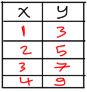
One critical step in the machine learning (ML) pipeline is to select the best algorithm that fits the data. Based on some statistics and visualizations from the data, the ML engineer will select the best algorithm. Let us apply that on a regression example with its data shown in figure 1.

Figure 1

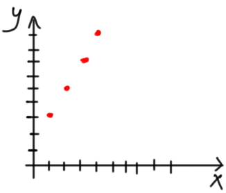
By visualizing the data according to figure 2, it seems that a linear regression model will be suitable.

Figure 2

A regression model with just one input and one output will be formulated according to the equation in figure 3.

Figure 3

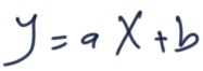
Where a and b are the parameters of the equation.

Because we do not know the optimal parameters that will fit the data, we can start with initial values. We can set a to 1.0 and b to 0.0 and visualize the model as in figure 4.

Figure 4

It seems that the model does not fit the data based on the initial values for the parameters.

It is expected that everything might not work from the first trial. The question is how to enhance the results in such cases? In other words, how to maximize the classification accuracy or minimize the regression error? There are different ways of doing that.

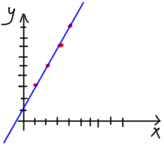
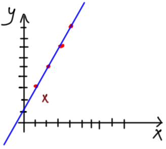
One simple way is to try to change the previously selected parameters. After a number of trials, the model will know that the optimal parameters are a=2 and b=1. The model will fit the data in such case as shown in figure 5. Very good.

Figure 5

But there are some cases in which changing the model parameters will not make the model fit the data. There will be some false predictions. Suppose that the data has a new point (x=2, y=2). According to figure 6, it is impossible to find parameters that make the model completely fits every data point.

Figure 6

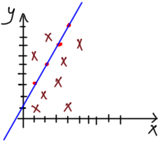
One might say that fitting 4 points and missing one is acceptable. But what if there are more points that the line can not fit as in figure 7? Thus the model will make more false predictions than the correct ones. There is no single line to fit the entire data. The model is strong in its predictions to the points on the line but weak for other points.

Figure 7

 

Ensemble Learning

 
Because a single regression model will not fit the entire data, an alternative solution is to use multiple regression models. Each regression model will be able to strongly fit a part of the data. The combination of all models will reduce the total error across the entire data and produce a generally strong model. Using multiple models in a problem is called ensemble learning. Importance of using multiple models is depicted in figure 8. Figure 8(a) shows that the error is high when predicting the outcome of the sample. According to figure 8(b), when there are multiple models (e.g. three models), the average of their outcomes will be able to make a more accurate prediction than before.

Figure 8

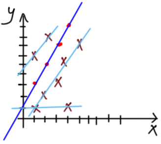
When being applied to the previous problem in figure 7, the ensemble of 4 regression models fitting the data is shown in figure 9.

Figure 9

This leaves another question. If there are multiple models to fit the data, how to get a single prediction? There are two ways to combine multiple regression models to return a single outcome. They are bagging and boosting (which is the focus of this tutorial).

In bagging, each model will return its outcome and the final outcome will be returned by summarizing all of such outcomes. One way is by averaging all outcomes. Bagging is parallel as all models are working at the same time.

In contrast, boosting is regarded sequential as the outcome of one model is the input to the next model. The idea of boosting is to use a weak learner to fit the data. Because it is weak, it will not be able to fit the data correctly. The weaknesses in such a learner will be fixed by another weak learner. If some weaknesses still exist, then another weak learner will be used to fix them. The chain got extended until finally producing a strong learner from multiple weak learners.

Next is to go through the explanation of how gradient boosting works.

 

Gradient Boosting (GB)

 
Here is how gradient boosting works based on a simple example:

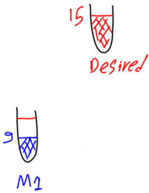
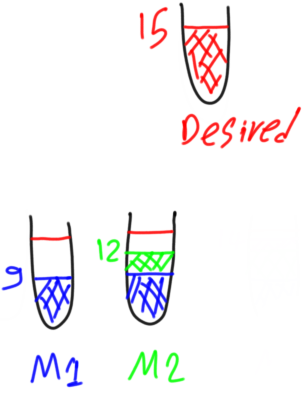
Suppose that a regression model is to be built and the data has a single output, where the first sample has an output 15. It is depicted as in figure 10. The goal is to build a regression model that correctly predict the output of such a sample.

Figure 10

The first weak model predicted the output of the first sample to be 9 rather than 15 as shown in figure 11.

Figure 11

To measure the amount of loss in the prediction, its residual is calculated. Residual is the difference between the desired and predicted outputs. It is calculated according to the following equation:

desired – predicted1 = residual1

Where predicted1 and residual1 are the predicted output and the residual of the first weak model, respectively.

By substituting by the values of the desired and predicted outputs, the residual will be 6:

15 – 9 = 6

For residual1=6 between the predicted and the desired outputs, we could create a second weak model where its target is to predict an output equal to the residual of the first model. Thus the second model will fix the weakness of the first model. The summation of the outputs from the two models will be equal to the desired output according to the next equation:

desired = predicted1 + predicted2(residual1)

If the second weak model was able to predict the residual1 correctly, then the desired output will equal the predictions of all weak models as follows:

desired = predicted1 + predicted2(residual1) = 9 + 6 = 15

But if the second weak model failed to correctly predict the value of residual1 and just returned 3 for example, then the second weak learner will also have a non-zero residual calculated as follows:

residual2 = predicted1 - predicted2 = 6 - 3 = 3

This is depicted in figure 12.

Figure 12

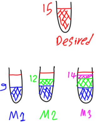
To fix the weakness of the second weak model, a third weak model will be created. Its goal is to predict the residual of the second weak model. Thus its target is 3. Thus the desired output of our sample will be equal to the predictions of all weak models as follows:

desired = predicted1 + predicted2(residual1) + predicted3(residual2)

If the third weak model prediction is 2, i.e. it is unable to predict the residual of the second weak model, then there will be a residual for such third model equal to as follows:

residual3 = predicted2 – predicted3 = 3 - 2 = 1

This is depicted in figure 13.

Figure 13

As a result, a fourth weak model will be created to predict the residual of the third weak model which equals to 1. The desired output will be equal to the predictions of all weak models as follows:

desired = predicted1 + predicted2(residual1) + predicted3(residual2) + predicted4(residual3)

If the fourth weak model predicted its target correctly (i.e. residual3), then the desired output of 15 has been reached using a total of four weak models as shown in figure 14.

Figure 14

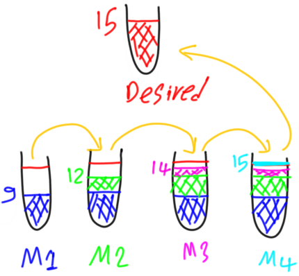
This is the core idea of the gradient boosting algorithm. Use the residuals of the previous model as the target of the next model.

 

Summary of GB

 
As a summary, gradient boosting starts with a weak model for making predictions. The target of such a model is the desired output of the problem. After training such model, its residuals are calculated. If the residuals are not equal to zero, then another weak model is created to fix the weakness of the previous one. But the target of such new model will not be the desired outputs but the residuals of the previous model. That is if the desired output for a given sample is T, then the target of the first model is T. After training it, there might be a residual of R for such sample. The new model to be created will have its target set to R, not T. This is because the new model fills the gaps of the previous models.

Gradient boosting is similar to lifting a heavy metal a number of stairs by multiple weak persons. No one of the weak persons is able to lift the metal all stairs. Each one can only lift it a single step. The first weak person will lift the metal one step and get tired after that. Another weak person will lift the metal another step, and so on until getting the metal lifted all stairs.

 
Bio: Ahmed Gad received his B.Sc. degree with excellent with honors in information technology from the Faculty of Computers and Information (FCI), Menoufia University, Egypt, in July 2015. For being ranked first in his faculty, he was recommended to work as a teaching assistant in one of the Egyptian institutes in 2015 and then in 2016 to work as a teaching assistant and a researcher in his faculty. His current research interests include deep learning, machine learning, artificial intelligence, digital signal processing, and computer vision.

Original. Reposted with permission.

Related:

• Introduction to Python Ensembles
• Building Convolutional Neural Network using NumPy from Scratch
• Ensemble Learning to Improve Machine Learning Results