Python Libraries for Interpretable Machine Learning

By Rebecca Vickery, Data Scientist

As concerns regarding bias in artificial intelligence become more prominent it is becoming more and more important for businesses to be able to explain both the predictions their models are producing and how the models themselves work. Fortunately, there is an increasing number of python libraries for data science being developed that attempt to solve this problem. In the following post, I am going to give a brief guide to four of the most established packages for interpreting and explaining machine learning models.

The following libraries are all pip installable, come with good documentation and have an emphasis on visual interpretation.

yellowbrick

This library is essentially an extension of the scikit-learn library and provides some really useful and pretty looking visualisations for machine learning models. The visualiser objects, the core interface, are scikit-learn estimators and so if you are used to working with scikit-learn the workflow should be quite familiar.

The visualisations that can be rendered cover model selection, feature importances and model performance analysis.

Let’s walk through a few brief examples.

The library can be installed via pip.

pip install yellowbrick

To illustrate a few features I am going to be using a scikit-learn dataset called the wine recognition set. This dataset has 13 features and 3 target classes and can be loaded directly from the scikit-learn library. In the below code I am importing the dataset and converting it to a data frame. The data can be used in a classifier without any additional preprocessing.

import pandas as pd
from sklearn import datasets
wine_data = datasets.load_wine()
df_wine = pd.DataFrame(wine_data.data,columns=wine_data.feature_names)
df_wine['target'] = pd.Series(wine_data.target)

I am also using scikit-learn to further split the data set into test and train.

from sklearn.model_selection import train_test_split
X = df_wine.drop(['target'], axis=1)
y = df_wine['target']
X_train, X_test, y_train, y_test = train_test_split(X, y, test_size=0.2)

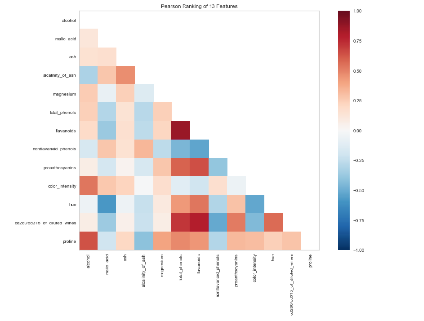
Next, let’s use the Yellowbricks visualiser to view correlations between features in the data set.

from yellowbrick.features import Rank2D
import matplotlib.pyplot as plt
visualizer = Rank2D(algorithm="pearson",  size=(1080, 720))
visualizer.fit_transform(X_train)
visualizer.poof()

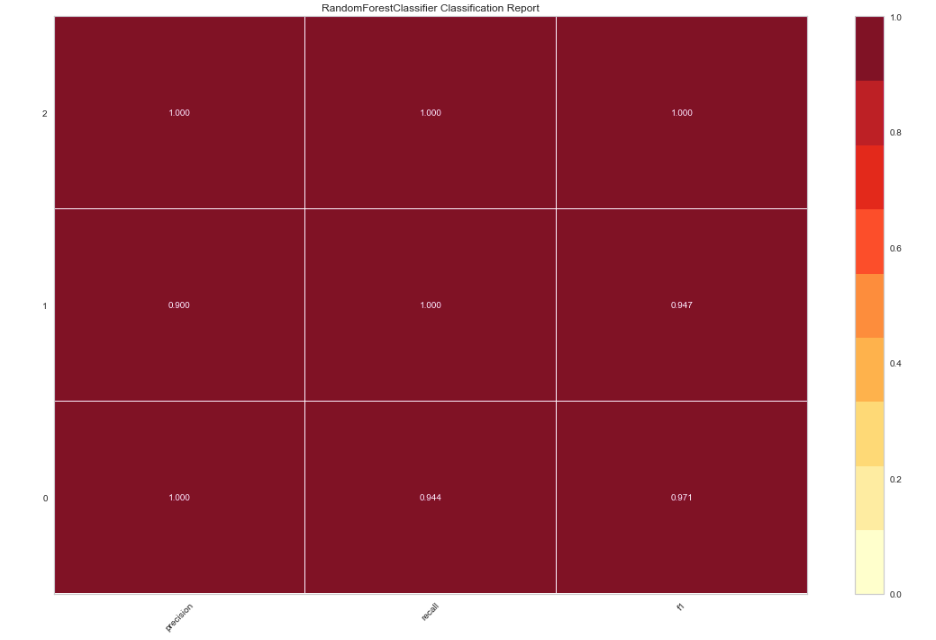
Let’s now fit a RandomForestClassifier and evaluate the performance with another visualiser.

from yellowbrick.classifier import ClassificationReport
from sklearn.ensemble import RandomForestClassifier
model = RandomForestClassifier()
visualizer = ClassificationReport(model, size=(1080, 720))
visualizer.fit(X_train, y_train)
visualizer.score(X_test, y_test)
visualizer.poof()

ELI5

ELI5 is another visualisation library that is useful for debugging machine learning models and explaining the predictions they have produced. It works with the most common python machine learning libraries including scikit-learn, XGBoost and Keras.

Let’s use ELI5 to inspect the feature importance for the model we trained above.

import eli5
eli5.show_weights(model, feature_names = X.columns.tolist())

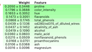
By default the show_weights method uses gain to calculate the weight but you can specify other types by adding the importance_type argument.

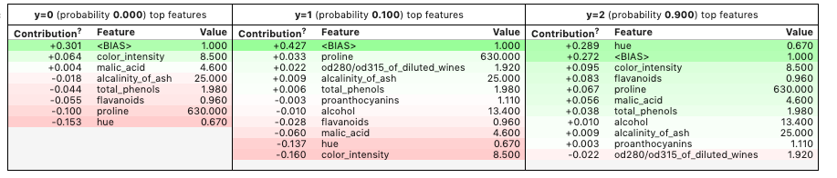
You can also use show_prediction to inspect the reasons for individual predictions.

from eli5 import show_prediction
show_prediction(model, X_train.iloc[1], feature_names = X.columns.tolist(), 
                show_feature_values=True)

LIME

LIME (local interpretable model-agnostic explanations) is a package for explaining the predictions made by machine learning algorithms. Lime supports explanations for individual predictions from a wide range of classifiers, and support for scikit-learn is built in.

Let’s use Lime to interpret some predictions from the model we trained earlier.

Lime can be installed via pip.

pip install lime

First, we build the explainer. This takes a training dataset as an array, the names of the features used in the model and the names of the classes in the target variable.

import lime.lime_tabular
explainer = lime.lime_tabular.LimeTabularExplainer(X_train.values,                                            
                 feature_names=X_train.columns.values.tolist(),                                        
                 class_names=y_train.unique())

Next, we create a lambda function that uses the model to predict on a sample of the data. This is borrowed from this excellent, more in-depth, tutorial on Lime.

predict_fn = lambda x: model.predict_proba(x).astype(float)

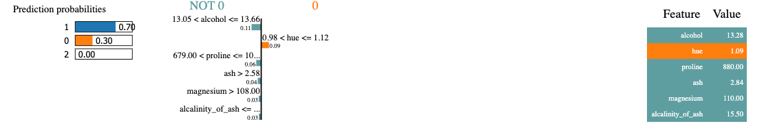
We then use the explainer to explain the prediction on a selected example. The result is shown below. Lime produces a visualisation showing how the features have contributed to this particular prediction.

exp = explainer.explain_instance(X_test.values[0], predict_fn, num_features=6)
exp.show_in_notebook(show_all=False)

MLxtend

This library contains a host of helper functions for machine learning. This covers things like stacking and voting classifiers, model evaluation, feature extraction and engineering and plotting. In addition to the documentation, this paper is a good resource for a more detailed understanding of the package.

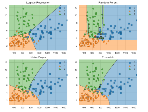
Let’s use MLxtend to compare the decision boundaries for a voting classifier against its constituent classifiers.

Again it can be installed via pip.

pip install mlxtend

The imports I am using are shown below.

from mlxtend.plotting import plot_decision_regions
from mlxtend.classifier import EnsembleVoteClassifier
import matplotlib.gridspec as gridspec
import itertoolsfrom sklearn import model_selection
from sklearn.linear_model import LogisticRegression
from sklearn.naive_bayes import GaussianNB
from sklearn.ensemble import RandomForestClassifier

The following visualisation only works with two features at a time so we will first create an array containing the features proline and color_intensity. I have chosen these as they had the highest weighting from all the features we inspected earlier using ELI5.

X_train_ml = X_train[['proline', 'color_intensity']].values
y_train_ml = y_train.values

Next, we create the classifiers, fit them to the training data and visualise the decision boundaries using MLxtend. The output is shown below the code.

clf1 = LogisticRegression(random_state=1)
clf2 = RandomForestClassifier(random_state=1)
clf3 = GaussianNB()
eclf = EnsembleVoteClassifier(clfs=[clf1, clf2, clf3], weights=[1,1,1])
value=1.5
width=0.75
gs = gridspec.GridSpec(2,2)
fig = plt.figure(figsize=(10,8))
labels = ['Logistic Regression', 'Random Forest', 'Naive Bayes', 'Ensemble']
for clf, lab, grd in zip([clf1, clf2, clf3, eclf],
                         labels,
                         itertools.product([0, 1], repeat=2)):
                         
    clf.fit(X_train_ml, y_train_ml)
    ax = plt.subplot(gs[grd[0], grd[1]])
    fig = plot_decision_regions(X=X_train_ml, y=y_train_ml, clf=clf)
    plt.title(lab)

This is by no means an exhaustive list of libraries for interpreting, visualising and explaining machine learning models. This excellent post contains a long list of other useful libraries to try out.
Thanks for reading!

Bio: Rebecca Vickery is learning data science through self study. Data Scientist @ Holiday Extras. Co-Founder of alGo.

Original. Reposted with permission.

Related:

• Opening Black Boxes: How to leverage Explainable Machine Learning
• A Data Science Playbook for explainable ML/xAI
• Command Line Basics Every Data Scientist Should Know