How to Build Your Own Logistic Regression Model in Python
A hands on guide to Logistic Regression for aspiring data scientist and machine learning engineer.
The name of this algorithm could be a little confusing in the sense that the Logistic Regression machine learning algorithm is for classification tasks and not regression problems. The name ‘Regression’ here implies that a linear model is fit into the feature space. This algorithm applies a logistic function to a linear combination of features to predict the outcome of a categorical dependent variable based on predictor variables. Logistic regression algorithms help estimate the probability of falling into a specific level of the categorical dependent variable based on the given predictor variables.
Suppose that you want to predict if there will be rain tomorrow in Toronto. Here the outcome of the prediction is not a continuous number because there will either be rain or no rain and hence linear regression cannot be applied. Here the outcome variable is one of the several categories and using logistic regression helps.
Applications of Logistic Regression
- Logistic regression algorithm is applied in the field of epidemiology to identify risk factors for diseases and plan accordingly for preventive measures.
- Used to predict whether a candidate will win or lose a political election or to predict whether a voter will vote for a particular candidate.
- Used in weather forecasting to predict the probability of rain.
- Used in credit scoring systems for risk management to predict the defaulting of an account.
Environment and tools
Where is the code?
Without much ado, let’s get started with the code. The complete project on github can be found here.
Let’s start with loading the libraries and dependencies.
import numpy as np
import matplotlib.pyplot as plt
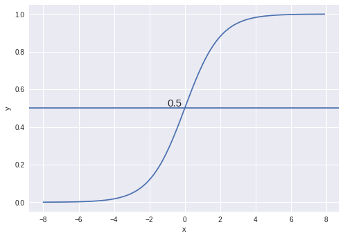
The first function is used for defining the sigmoid activation function. The plot of the sigmoid function looks like this:
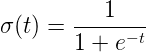
def sigmoid(scores):
   return 1 / (1 + np.exp(-scores))
The sigmoid function is represented as shown:
The sigmoid function also called the logistic function gives an ‘S’ shaped curve that can take any real-valued number and map it into a value between 0 and 1. If the curve goes to positive infinity, y predicted will become 1, and if the curve goes to negative infinity, y predicted will become 0. If the output of the sigmoid function is more than 0.5, we can classify the outcome as 1 or yes, and if it is less than 0.5, we can classify it like 0 or no.
The next function is used for returning the log likelihood value. The parameters associated with this function are feature vectors, target value and weights of the model.
The log-likelihood is as the term suggests, the natural logarithm of the likelihood. In turn, given a sample and a parametric family of distributions (i.e., a set of distributions indexed by a parameter) that could have been generated from the sample the likelihood is a function that associates to each parameter the probability of observing the given sample.
def log_likelihood(features, target, weights):
   scores = np.dot(features, weights)
   ll = np.sum(target * scores - np.log(1 + np.exp(scores)))
   return ll
The next function is used to make the logistic regression model. The parameters associated with this function are feature vectors, target value, number of steps for training, learning rate and a parameter for adding intercept which is set to false by default.
First weights are assigned using feature vectors. Next score is calculated using dot product of feature and weight vectors. The prediction is found by applying the sigmoid function to the score. Now error can be calculated which is the difference between target and prediction values. This error is used for finding out the gradient which is the dot product of transposed feature vector and error. The new weights can be calculated by adding learning rate multiplied by gradient to the old weights.
def logistic_regression(features, target, num_steps, learning_rate, add_intercept=False):
    if add_intercept:
       intercept = np.ones((features.shape[0], 1))
       features = np.hstack((intercept, features))     weights = np.zeros(features.shape[1])

    for step in range(num_steps):
      scores = np.dot(features, weights)
      predictions = sigmoid(scores)
      output_error_signal = target - predictions
      gradient = np.dot(features.T, output_error_signal)
      weights += learning_rate * gradient

      if step % 10000 == 0:
        print(log_likelihood(features, target, weights))

return weights
random() function is used to generate random numbers in Python. Seed function is used to save the state of random function, so that it can generate some random numbers on multiple execution of the code on the same machine or on different machines. The seed value chosen is 10 with 10000 data points.
The multivariate normal is a generalization of the one-dimensional normal distribution to higher dimensions. Such a distribution is specified by its mean and covariance matrix.
np.random.seed(10)
num_observations = 10000 x1 = np.random.multivariate_normal([0, 0], [[1, 0.5], [0.5, 1]], num_observations)
x2 = np.random.multivariate_normal([1, 4], [[1, 0.5], [0.5, 1]], num_observations)
hstack is used for appending data horizontally while vstack is used for appending data vertically. First vstack is used to separate the data points using features and then hstack is used for separating the data points using labels.
simulated_separableish_features = np.vstack((x1, x2)).astype(np.float32)simulated_labels = np.hstack((np.zeros(num_observations), np.ones(num_observations)))
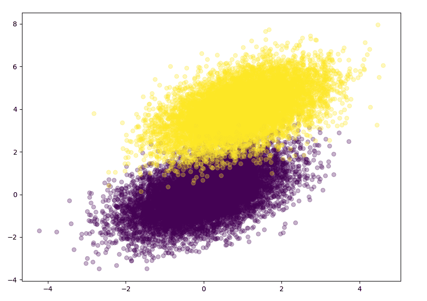
Let’s visualize the results by plotting the separated data points using scatter function where alpha blending value is chosen to be 0.3. The blending value can range between 0 (transparent) and 1 (opaque).
plt.figure(figsize=(10, 8))plt.scatter(simulated_separableish_features[:, 0],   simulated_separableish_features[:, 1], c=simulated_labels,    alpha=0.3,)

plt.show()
Results
Conclusions
To conclude, I demonstrated how to make a logistic regression model from scratch in python. Logistic regression is a widely used supervised machine learning technique. It is one of the best tools for statisticians, researchers and data scientists in predictive analytics. It offers several advantages like it is a robust algorithm as the independent variables need not have equal variance or normal distribution, do not assume a linear relationship between the dependent and independent variables and hence can also handle non-linear effects and they are also easier to inspect and less complex.
References/Further Readings
Logistic Regression — Detailed Overview
Logistic Regression was used in the biological sciences in early twentieth century. It was then used in many social…
Tips for honing your logistic regression models | Zopa Blog
When we create our Credit Risk assessment or Fraud prevention machine learning models at Zopa, we use a variety of…
Before You Go
The corresponding source code can be found here.
Contacts
If you want to keep updated with my latest articles and projects follow me on Medium. These are some of my contacts details:
Happy reading, happy learning and happy coding.
Bio: Abhinav Sagar is a senior year undergrad at VIT Vellore. He is interested in data science, machine learning and their applications to real-world problems.
Original. Reposted with permission.
Related:
- Logistic Regression: A Concise Technical Overview
- Convolutional Neural Network for Breast Cancer Classification
- How to Easily Deploy Machine Learning Models Using Flask