Building Predictive Models: Logistic Regression in Python
Want to learn how to build predictive models using logistic regression? This tutorial covers logistic regression in depth with theory, math, and code to help you build better models.
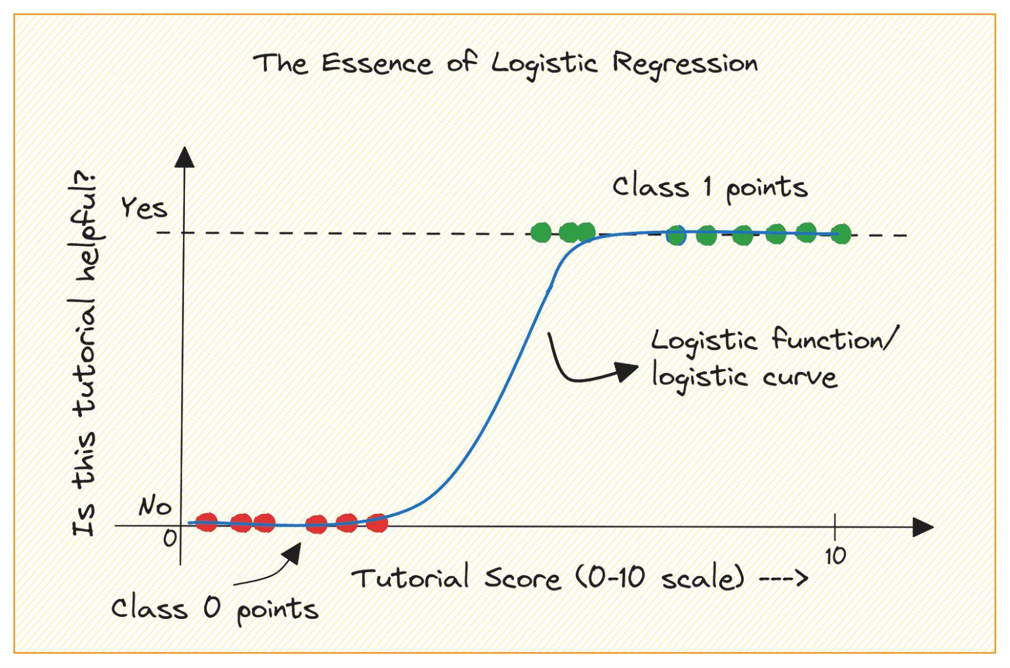
Image by Author
When you are getting started with machine learning, logistic regression is one of the first algorithms you’ll add to your toolbox. It's a simple and robust algorithm, commonly used for binary classification tasks.
Consider a binary classification problem with classes 0 and 1. Logistic regression fits a logistic or sigmoid function to the input data and predicts the probability of a query data point belonging to class 1. Interesting, yes?
In this tutorial, we’ll learn about logistic regression from the ground up covering:
- The logistic (or sigmoid) function
- How we move from linear to logistic regression
- How logistic regression works
Finally, we’ll build a simple logistic regression model to classify RADAR returns from the ionosphere.
Logistic Function
Before we learn more about logistic regression, let's review how the logistic function works. The logistic (or sigmoid function) is given by:

When you plot the sigmoid function, it’ll look like so:
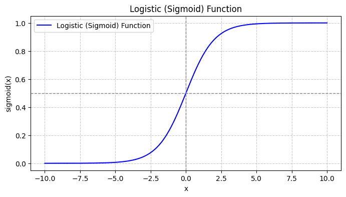
From the plot, we see that:
- When x = 0, σ(x) takes a value of 0.5.
- When x approaches +∞, σ(x) approaches 1.
- When x approaches -∞, σ(x) approaches 0.
So for all real inputs, the sigmoid function squishes them to take on values in the range [0, 1].
From Linear Regression to Logistic Regression
Let's first discuss why we cannot use linear regression for a binary classification problem.
In a binary classification problem, the output is categorical label (0 or 1). Because linear regression predicts continuous-valued outputs which can be less than 0 or greater than 1, it does not make sense for the problem at hand.
Also, a straight line may not be the best fit when the output labels belong to one of the two categories.

Image by Author
So how do we go from linear to logistic regression? In linear regression the predicted output is given by:

Where the βs are the coefficients and X_is are the predictors (or features).
Without loss of generality, let’s assume X_0 = 1:

So we can have a more concise expression:

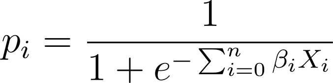
In logistic regression, we need the predicted probability p_i in the [0,1] interval. We know that the logistic function squishes inputs so that they take on values in the [0,1] interval.
So plugging in this expression into the logistic function, we have the predicted probability as:
Under the Hood of Logistic Regression
So how do we find the best fit logistic curve for the given data set? To answer this, let’s understand maximum likelihood estimation.
Maximum Likelihood Estimation (MLE) is used to estimate the parameters of the logistic regression model by maximizing the likelihood function. Let's break down the process of MLE in logistic regression and how the cost function is formulated for optimization using gradient descent.
Breaking Down Maximum Likelihood Estimation
As discussed, we model the probability that a binary outcome occurs as a function of one or more predictor variables (or features):
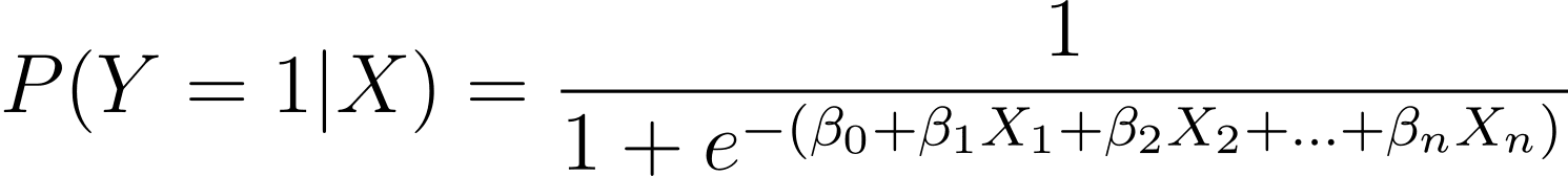
Here, the βs are the model parameters or coefficients. X_1, X_2,..., X_n are the predictor variables.
MLE aims to find the values of β that maximize the likelihood of the observed data. The likelihood function, denoted as L(β), represents the probability of observing the given outcomes for the given predictor values under the logistic regression model.
Formulating the Log-Likelihood Function
To simplify the optimization process, it's common to work with the log-likelihood function. Because it transforms products of probabilities into sums of log probabilities.
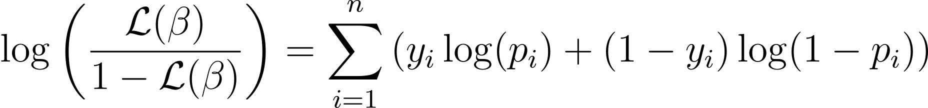
The log-likelihood function for logistic regression is given by:
Cost Function and Gradient Descent
Now that we know the essence of log-likelihood, let's proceed to formulate the cost function for logistic regression and subsequently gradient descent for finding the best model parameters
Cost Function for Logistic Regression
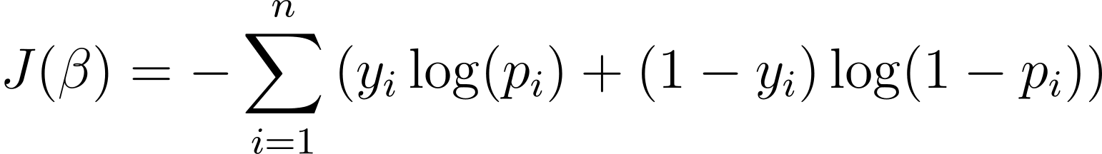
To optimize the logistic regression model, we need to maximize the log-likelihood. So we can use the negative log-likelihood as the cost function to minimize during training. The negative log-likelihood, often referred to as the logistic loss, is defined as:
The goal of the learning algorithm, therefore, is to find the values of ? that minimize this cost function. Gradient descent is a commonly used optimization algorithm for finding the minimum of this cost function.
Gradient Descent in Logistic Regression
Gradient descent is an iterative optimization algorithm that updates the model parameters β in the opposite direction of the gradient of the cost function with respect to β. The update rule at step t+1 for logistic regression using gradient descent is as follows:
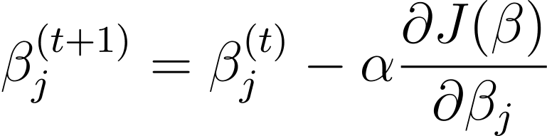
Where α is the learning rate.
The partial derivatives can be computed using the chain rule. Gradient descent iteratively updates the parameters—until convergence—aiming to minimize the logistic loss. As it converges, it finds the optimal values of β that maximize the likelihood of the observed data.
Logistic Regression in Python with Scikit-Learn
Now that you know how logistic regression works, let’s build a predictive model using the scikit-learn library.
We’ll use the ionosphere dataset from the UCI machine learning repository for this tutorial. The dataset comprises 34 numerical features. The output is binary, one of ‘good’ or ‘bad’ (denoted by ‘g’ or ‘b’). The output label ‘good’ refers to RADAR returns that have detected some structure in the ionosphere.
Step 1 – Loading the Dataset
First, download the dataset and read it into a pandas dataframe:
import pandas as pd
import urllib

url = "https://archive.ics.uci.edu/ml/machine-learning-databases/ionosphere/iphere.data"
data = urllib.request.urlopen(url)
df = pd.read_csv(data, header=None)
Step 2 – Exploring the Dataset
Let's take a look at the first few rows of the dataframe:
# Display the first few rows of the DataFrame
df.head()
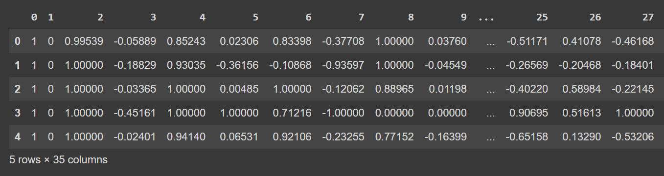
Truncated Output of df.head()
Let's get some information about the dataset: the number of non-null values and the data types of each of the columns:
# Get information about the dataset
print(df.info())
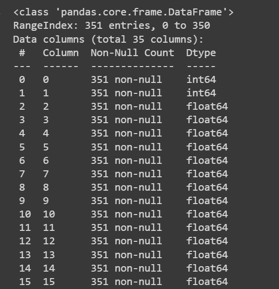 Truncated Output of df.info()
Because we have all numeric features, we can also get some descriptive statistics using the describe() method on the dataframe:
# Get descriptive statistics of the dataset
print(df.describe())
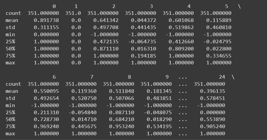
Truncated Output of df.describe()
The column names are currently 0 through 34—including the label. Because the dataset does not provide descriptive names for the columns, it just refers to them as attribute_1 to attribute_34 if you would like you can rename the columns of the data frame as shown:
column_names = [
"attribute_1", "attribute_2", "attribute_3", "attribute_4", "attribute_5",
"attribute_6", "attribute_7", "attribute_8", "attribute_9", "attribute_10",
"attribute_11", "attribute_12", "attribute_13", "attribute_14", "attribute_15",
"attribute_16", "attribute_17", "attribute_18", "attribute_19", "attribute_20",
"attribute_21", "attribute_22", "attribute_23", "attribute_24", "attribute_25",
"attribute_26", "attribute_27", "attribute_28", "attribute_29", "attribute_30",
"attribute_31", "attribute_32", "attribute_33", "attribute_34", "class_label"
]
df.columns = column_names
Note: This step is purely optional. You can proceed with the default column names if you prefer.
# Display the first few rows of the DataFrame
df.head()
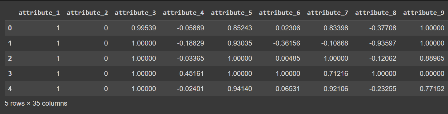
Truncated Output of df.head() [After Renaming Columns]
Step 3 – Renaming Class Labels and Visualizing Class Distribution
Because the output class labels are ‘g’ and ‘b’, we need to map them to 1 and 0 , respectively. You can do it using map() or replace():
# Convert the class labels from 'g' and 'b' to 1 and 0, respectively
df["class_label"] = df["class_label"].replace({'g': 1, 'b': 0})
Let’s also visualize the distribution of the class labels:
import matplotlib.pyplot as plt

# Count the number of data points in each class
class_counts = df['class_label'].value_counts()

# Create a bar plot to visualize the class distribution
plt.bar(class_counts.index, class_counts.values)
plt.xlabel('Class Label')
plt.ylabel('Count')
plt.xticks(class_counts.index)
plt.title('Class Distribution')
plt.show()
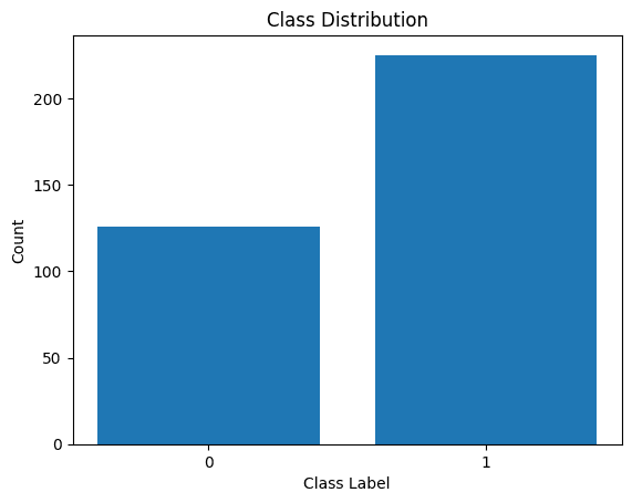
Distribution of Class Labels
We see that there is an imbalance in the distribution. There are more records belonging to class 1 than to class 0. We’ll handle this class imbalance when building the logistic regression model.
Step 5 – Preprocessing the Dataset
Let’s collect the features and output labels like so:
X = df.drop('class_label', axis=1)  # Input features
y = df['class_label']               # Target variable
After splitting the dataset into the train and test sets, we need to preprocess the dataset.
When there are many numeric features—each on a potentially different scale—we need to preprocess the numeric features. A common method is to transform them such that they follow a distribution with zero mean and unit variance.
The StandardScaler from scikit-learn’s preprocessing module helps us achieve this.
from sklearn.preprocessing import StandardScaler
from sklearn.model_selection import train_test_split

# Split the dataset into training and testing sets
X_train, X_test, y_train, y_test = train_test_split(X, y, test_size=0.2, random_state=42)

# Get the indices of the numerical features
numerical_feature_indices = list(range(34))  # Assuming the numerical features are in columns 0 to 33

# Initialize the StandardScaler
scaler = StandardScaler()

# Normalize the numerical features in the training set
X_train.iloc[:, numerical_feature_indices] = scaler.fit_transform(X_train.iloc[:, numerical_feature_indices])

# Normalize the numerical features in the test set using the trained scaler from the training set
X_test.iloc[:, numerical_feature_indices] = scaler.transform(X_test.iloc[:, numerical_feature_indices])
Step 6 – Building a Logistic Regression Model
Now we can instantiate a logistic regression classifier. The LogisticRegression class is part of scikit-learn’s linear_model module.
Notice that we have set the class_weight parameter to ‘balanced’. This will help us account for the class imbalance. By assigning weights to each class—inversely proportional to the number of records in the classes.
After instantiating the class, we can fit the model to the training dataset:
from sklearn.linear_model import LogisticRegression

model = LogisticRegression(class_weight='balanced')
model.fit(X_train, y_train)
Step 7 – Evaluating the Logistic Regression Model
You can call the predict() method to get the model’s predictions.
In addition to the accuracy score, we can also get a classification report with metrics like precision, recall, and F1-score.
from sklearn.metrics import accuracy_score, classification_report

y_pred = model.predict(X_test)
accuracy = accuracy_score(y_test, y_pred)
print(f"Accuracy: {accuracy:.2f}")

classification_rep = classification_report(y_test, y_pred)
print("Classification Report:\n", classification_rep)
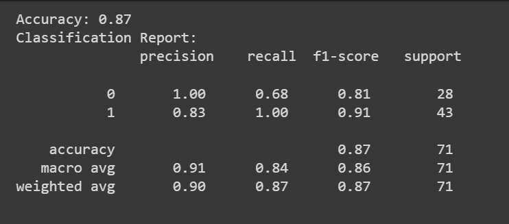
Congratulations, you have coded your first logistic regression model!
Conclusion
In this tutorial, we learned about logistic regression in detail: from theory and math to coding a logistic regression classifier.
As a next step, try building a logistic regression model for a suitable dataset of your choice.
Dataset Credits
The Ionosphere dataset is licensed under a Creative Commons Attribution 4.0 International (CC BY 4.0) license:
Sigillito,V., Wing,S., Hutton,L., and Baker,K.. (1989). Ionosphere. UCI Machine Learning Repository. https://doi.org/10.24432/C5W01B.
Bala Priya C is a developer and technical writer from India. She likes working at the intersection of math, programming, data science, and content creation. Her areas of interest and expertise include DevOps, data science, and natural language processing. She enjoys reading, writing, coding, and coffee! Currently, she's working on learning and sharing her knowledge with the developer community by authoring tutorials, how-to guides, opinion pieces, and more. Bala also creates engaging resource overviews and coding tutorials.