Writing Your First Neural Net in Less Than 30 Lines of Code with Keras

By David Gündisch, Cloud Architect

https://unsplash.com/@tvick

Reminiscing back to when I first started my journey into AI, I remember all too well how daunting some of the concepts seemed. Reading a simple explanation on what a Neural Network is can quickly lead to a scientific paper where every second sentence is a formula with symbols you’ve never even seen before. While these papers hold incredible insights and depth to help you build up your expertise, getting started with writing your first Neural Net is a lot easier than it sounds!

OK… but what even is a Neural Network???

 
Good Question! Before we jump into writing our own Python implementation of a simple Neural Network or NN for short, we should probably unpack what they are, and why they are so exciting!

Dr. Robert Hecht-Nielsen, co-founder of HNC Software, puts it simply.

…a computing system made up of a number of simple, highly interconnected processing elements, which process information by their dynamic state response to external inputs. — “Neural Network Primer: Part I” by Maureen Caudill, AI Expert, Feb. 1989

In essence, a Neural Network is a set of mathematical expressions that are really good at recognizing patterns in information, or data. A NN accomplishes this through a kind of human emulated perception, but instead of seeing, say an image, like a human would, the NN expresses this information numerically contained within a Vector or Scalar (a Vector only containing one number).

It passes this information through layers where the output of one layer, acts as the input into the next. While traveling through these layers the input is modified by weight and bias and sent to the activation function to map the output. The learning then occurs via a Cost function, that compares the actual output and the desired output, which in turn helps the function alters and adjusts the weights and biases to minimize the cost via a process called backpropagation.

I would highly encourage you to watch the below video for an in-depth and visual explanation.

For our example NN implementation we are going to be using the MNIST data set.

MNIST Sample Dataset

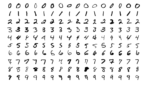
MNIST can be seen as the ‘Hello World’ dataset because it is able to demonstrate the capabilities of NNs quite succinctly. The dataset is made up of handwritten digits, which we will train our NN to recognize and classify.

Enter the drago… I mean Keras

 
To facilitate our implementation we are going to be using the Keras framework. Keras is a high-level API written in Python which runs on-top of popular frameworks such as TensorFlow, Theano, etc. to provide the machine learning practitioner with a layer of abstraction to reduce the inherent complexity of writing NNs.

I would encourage you to delve into the Keras documentation to really become familiar with the API. Additionally, I would highly recommend the book Deep Learning with Python by Francois Chollet, which inspired this tutorial.

Time to burn some GPUs

 
For this tutorial, we will be using Keras with the TensorFlow backend, so if you haven’t installed either of these, now is a good time to do so. You can accomplish this simply by running these commands in your terminal. When you move beyond simple introductory examples it is best to set up your Anaconda environment and install the below with conda instead.

pip3 install Keras
pip3 install Tensorflow

Now that you’ve installed everything standing between you and your first NN, go ahead and open your favorite IDE and let’s dive into importing our required Python modules!

from keras.datasets import mnist
from keras import models
from keras import layers
from keras.utils import to_categorical

Keras has a number of datasets you can use to help you learn and luckily for us MNIST is one of them! Models and Layers are both modules which will help us build out our NN and to_categorical is used for our data encoding… but more on that later!

Now that we have our required modules imported we will want to split our dataset into train and test sets. This can be accomplished simply with the following line.

(train_images, train_labels), (test_images, test_labels) = mnist.load_data()

In this example, our NN learns by comparing its output against labeled data. You can think of this as us making the NN guess a large number of handwritten digits, and then comparing the guesses against the actual label. The result of this will then feed into how the model adjusts its weights and biases in order to minimize the overall cost.

With our training and test data set-up, we are now ready to build our model.

network = models.Sequential()
network.add(layers.Dense(784, activation='relu', input_shape=(28 * 28,)))
network.add(layers.Dense(784, activation='relu', input_shape=(28 * 28,)))network.add(layers.Dense(10, activation='softmax'))network.compile(optimizer='adam',
                loss='categorical_crossentropy',
                metrics=['accuracy'])

I know… I know… it might seem like a lot, but let’s break it down together! We initialize a sequential model called network.

network = models.Sequential()

And we add our NN layers. For this example, we will be using dense layers. A dense layer simply means that each neuron receives input from all the neurons in the previous layer. [784] and [10] refer to the dimensionality of the output space, we can think of this as the number of inputs for the subsequent layers, and since we are trying to solve a classification problem with 10 possible categories (numbers 0 to 9) the final layer has a potential output of 10 units. The activation parameter refers to the activation function we want to use, in essence, an activation function calculates an output based on a given input. And finally, the input shape of [28 * 28] refers to the image’s pixel width and height.

network.add(layers.Dense(784, activation='relu', input_shape=(28 * 28,)))
network.add(layers.Dense(784, activation='relu', input_shape=(28 * 28,)))
network.add(layers.Dense(10, activation='softmax'))

Once our model is defined, and we have added our NN layers, we simply compile the model with our optimizer of choice, our loss function of choice, and the metrics we want to use to judge our model’s performance.

network.compile(optimizer='adam',
                loss='categorical_crossentropy',
                metrics=['accuracy'])

Congratulations!!! You’ve just built your first Neural Network!!

Now you still might have some questions, such as; What are relu and softmax? and Who the hell is adam? And those are all valid questions… An in-depth explanation of these falls slightly out of scope for our initial journey into NN but we will cover these in later posts.

Before we can feed our data into our newly created model we will need to reshape our input into a format that the model can read. The original shape of our input was [60000, 28, 28] which essentially represents 60000 images with a pixel height and width of 28 x 28. We can reshape our data and split it between train [60000] images and test [10000] images.

train_images = train_images.reshape((60000, 28 * 28))
train_images = train_images.astype('float32') / 255
test_images = test_images.reshape((10000, 28 * 28))
test_images = test_images.astype('float32') / 255

In addition to reshaping our data, we will also need to encode it. For this example, we will use categorical encoding, which in essence turns a number of features in numerical representations.

train_labels = to_categorical(train_labels)
test_labels = to_categorical(test_labels)

With our dataset split into a training and test set, with our model compiled and with our data reshaped and encoded, we are now ready to train our NN! To do this we will call the fit function and pass in our required parameters.

network.fit(train_images, train_labels, epochs=5, batch_size=128)

We pass in our training images and their labels as well as epochs, which dictate the number of backward and forward propagations, and the batch_size, which indicates the number of training samples per backward/forward propagation.

We will also want to set our performance measuring parameters so we can identify how well our model is working.

test_loss, test_acc = network.evaluate(test_images, test_labels)
print('test_acc:', test_acc, 'test_loss', test_loss)

And voila!!! You have just written your own Neural Network, reshaped and encoded a dataset and fit your model to train! When you run the Python script for the first time Keras will download the MNIST dataset and begin training for 5 epochs!

Training cycle with Test output

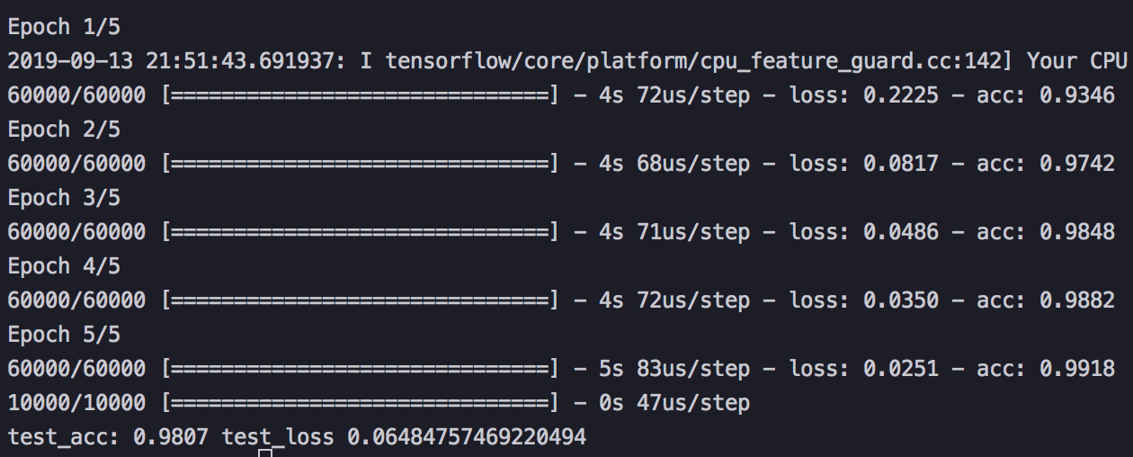
You should get an accuracy of around 98 percent for your test accuracy, which means that the model has predicted the correct digit 98 percent of the time while running its tests, not bad for your first NN! In practice, you’ll want to look at both the testing and training results to get a good idea if your model is overfitted/underfitted.

I’d encourage you to play around with the number of layers, the optimizer and loss function, as well as the epoch and batch_size to see what the impact of each would be to your model’s overall performance!

You’ve just taken the difficult first step in your long and exciting learning journey! Feel free to reach out for any additional clarification or feedback!

Thanks for reading — and stay curious! ????

 
Bio: David Gündisch is a Cloud Architect. He is passionate about researching the applications of Artificial Intelligence within the fields of Philosophy, Psychology and Cyber Security.

Original. Reposted with permission.

Related:

• Introduction to Artificial Neural Networks
• A Gentle Introduction to PyTorch 1.2
• TensorFlow vs PyTorch vs Keras for NLP