A Gentle Introduction to PyTorch 1.2
This comprehensive tutorial aims to introduce the fundamentals of PyTorch building blocks for training neural networks.
By Elvis Saravia, Affective Computing & NLP Researcher
In our previous PyTorch notebook, we learned about how to get started quickly with PyTorch 1.2 using Google Colab. In this tutorial, we are going to take a step back and review some of the basic components of building a neural network model using PyTorch. As an example, we will build an image classifier using a few stacked layers and then evaluate the model.
This will be a brief tutorial and will avoid using jargon and over-complicated code. That said, this is perhaps the most basic of neural network models you can build with PyTorch.
If fact, it is so basic that it’s ideal for those starting to learn about PyTorch and machine learning. So if you have a friend or colleague that wants to jump in, I highly encourage you to refer them to this tutorial as a starting point. Let’s get started!
Getting Started
Before you get started with code, you need to install the latest version of PyTorch. We are using Google Colab for our tutorial, so we will use the following command to install PyTorch. You can also find a Colab notebook towards the end of this blog post.
Now we need to import a few modules which will be useful to obtain the necessary functions that will help us to build our neural network model. The main ones are torch and torchvision. They contain the majority of the functions that you need to get started with PyTorch. However, as this is a machine learning tutorial we will need torch.nn, torch.nn.functional and torchvision.transforms which all contain utility functions to build our model. We probably won't use all the modules listed below but they are the typical modules you will need to import before starting your machine learning projects.
Below we check for the PyTorch version just to make sure that you are using the proper version that was used for this tutorial. At the time of this tutorial, we are working with PyTorch 1.2.
print(torch.__version__)
Loading the Data
Let’s get right into it! As with any machine learning project, you need to load your dataset. We are using the MNIST dataset, which is the “Hello World” of datasets in the machine learning world.
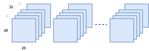
The data consists of a series of images (containing hand-written numbers) that are of the size 28 X 28. We will discuss the images shortly, but our plan is to load the data into batches of 32, similar to the figure below:
Here are the complete steps we are performing when importing our data:
- We will import and transform the data into tensors using the
transformsmodule. In the context of machine learning, tensors are just efficient data structures used to store data. - We will use
DataLoaderto build convenient data loaders, which makes it easy to efficiently feed data in batches to neural network models. We will get to the topic of batches in a bit but for now, just think of them as subsets of your data. - As hinted above, we will also create batches of the data by setting the
batchparameter inside the data loader. Notice we use batches of32in this tutorial but you can change it to64if you like.
Let’s inspect what the trainset and testset objects contain.
print(trainset)print(testset)## outputDataset MNIST
Number of datapoints: 60000
Root location: ./data
Split: Train
StandardTransform
Transform: Compose(ToTensor()) Dataset MNIST
Number of datapoints: 10000
Root location: ./data
Split: Test
StandardTransform Transform: Compose(ToTensor())
This is a beginner’s tutorial so I will break down things a bit here:
BATCH_SIZEis a parameter that denotes the batch size we will use for our modeltransformholds code for whatever transformations you will apply to your data. I will show you an example below to demonstrate exactly what it does to shed more light into its usetrainsetandtestsetcontain the actual dataset object. Notice I usetrain=Trueto specify that this corresponds to the training dataset, and I usetrain=Falseto specify that this is the remainder of the dataset which we call the test set. From the block I printed above you can see that the split of the data was 85% (60000) / 15% (10000), corresponding to the portions of samples for the training set and testing set, respectivelytrainloaderis what holds the data loader object which takes care of shuffling the data and constructing the batches
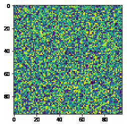
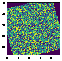
Now let’s take a closer look at that transforms.Compose(...) function and see what it does. We will use a randomly generated image to demonstrate its use. Let's generate an image:
And let’s render it:
The output:
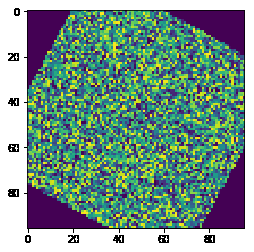
Okay, we have our image sample, so now let’s apply some dummy transformation to it. We are going to rotate the image by 45 degrees. The transformation below takes care of that:
The output:
Notice you can put any transformations within transforms.Compose(...). You can use the built-in transformations offered by PyTorch or you can build your own and compose transformations as you wish. In fact, you can place as many transformations in the function as you wish. Let's try another composition of transformations: rotate + vertical flip.
The output:
That’s pretty cool right! Keep trying other transform methods. On the topic of exploring our data further, let’s take a closer look at our images dataset.
Exploring the Data
As a practitioner and researcher, I always spend a bit of time and effort exploring and understanding my datasets. It’s fun and this is a good practice to ensure that everything is in order before training the model.
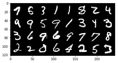
Let’s check what the train and test dataset contains. I will use the matplotlib library to print out some of the images from our dataset. With a bit of numpy code, I can convert images into a proper format to print them out. Below I print out an entire batch of 32 images:
The output:
The dimensions of our batches are as follows:
The output:
Image batch dimensions: torch.Size([32, 1, 28, 28])
Image label dimensions: torch.Size([32])
The Model
Now it’s time to build the neural network model that will be used to perform the image classification task. We will keep things simple and stack a dense layer, a dropout layer, and an output layer to train our model.
Let’s discuss a bit about the model:
- First of all, the following structure, involving a
classcalledMyModel, is standard code that's used to build a neural network model in PyTorch:
- The layers are defined inside the
def __init__()function.super(...).__init__()is just there to stick things together. For our model, we stack a hidden layer (self.d1) followed by a dropout layer (self.dropout), which is then followed by an output layer (self.d2). nn.Linear(...)defines the dense layer and it requires theinandoutdimensions, which corresponds to the size of the input feature and output feature of that layer, respectively.nn.Dropout(...)is used to define a dropout layer. Dropout is an approach in deep learning that helps a model to avoid overfitting. This means that dropout acts as a regularization technique that helps the model to not overfit on the images it has seen while training. We want this because we need a model that generalizes well to unseen examples — in our case, the testing dataset. Dropout randomly zeroes some of the units of the neural network layer with the probability ofp=0.2. Read more about the dropout layer here.- The entry point of the model, i.e. where the data is fed into the neural network model, is placed under the
forward(...)function. Typically, we also place other transformations we perform on the data while training inside this function. - In the
forward()function, we are performing a series of computations on the input data: 1) we flatten the images first, converting it from 2D (28 X 28) to 1D (1 X 784); 2) then we feed the batches of those 1D images into the first hidden layer; 3) the output of that hidden layer is then applied a non-linear activate function calledReLU. It's not so important to know whatF.relu()does at the moment, but the effect that it achieves is that it allows faster and more effective training of neural architectures on large datasets; 4) as explained above, the dropout also helps the model to train more efficiently by avoiding overfitting on the training data; 5) we then feed the output of that dropout layer into the output layer (d2); 6) the result of that is then fed to the softmax function, which converts or normalizes the output into a probability distribution which helps with outputting proper prediction values that are used to calculate the accuracy of the model; 7) this will be the final output of the model.
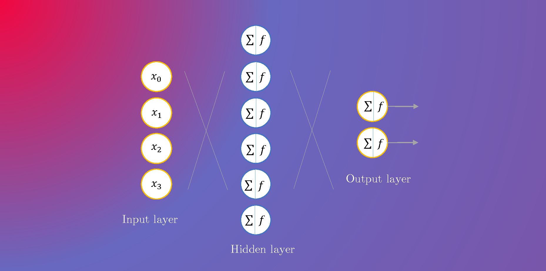
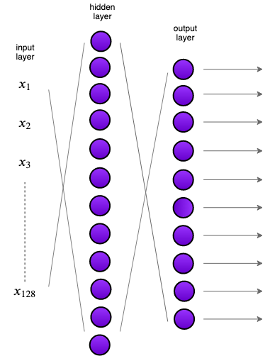
Visually speaking, the following is a diagram of the model that we have just built. Just keep in mind that the hidden layer is much bigger than shown in the diagram but due to space constraint, the diagram should be viewed as an approximation of the actual model.
As I have done in my previous tutorials, I always encourage to test the model with one batch to ensure that the dimensions of the output are what we expect. Notice how we are iterating over the dataloader which conveniently stores the images and labels pairs. out contains the output of the model, which are the logits applied a softmax layer which helps with prediction.
The output:
batch size: torch.Size([32, 1, 28, 28])
torch.Size([32, 10])
We can clearly see that we get back the batches with 10 output values associated with each image in the batch; these values are used to check the performance of the model.
Training the Model
Now we are ready to train the model but before that, we are going to set up a loss function, an optimizer, and a utility function to calculate the accuracy of the model:
- The
learning_rateis the rate at which the model will try to optimize its weights, so it can be seen as just another parameter of the model. num_epochsis the number of training steps… we don’t need to train this model for long so we just use 5 epochs.devicedetermines what hardware we will use to train the model. If agpuis present, then that will be used, otherwise, it defaults to thecpu.modelis just the model instance.model.to(device)is in charge of setting the actual device that will be used for training the model.criterionis just the metric that's used to compute the loss of the model while it forward and backward trains to optimize its weights.optimizeris the optimization technique used to modify the weights in the backward propagation step. Notice that it requires thelearning_rateand the model parameters which are part of the optimization. More on this in a bit!
The utility function below helps to calculate the accuracy of the model. For now, it’s not important to understand how it’s calculated but basically it compares the outputs of the model (predictions) with the actual target values (i.e., the labels of the dataset), and tries to compute the average of correct predictions.
Training the Model
Now it’s time to train the model. The code portion that follows can be described in the following steps:
- The first thing when training a neural network model is defining the training loop, which is achieved by:
for epoch in range(num_epochs):
    ...
- We define two variables,
training_running_lossandtrain_acc, that will help us to monitor the running accuracy and loss of the model while it trains over the different batches. model.train()explicitly indicates that we are ready to start training.- Notice that we are iterating over the dataloader, which conveniently gives us the batches in image-label pairs.
- That second
forloop means that for every training step we will iterate over all the batches and train the model over them. - We feed the model the images via
model(images)and the output represents the predictions of the model. - The predictions together with the target labels are used to compute the loss using the loss function we defined earlier.
- Before we update our weights for the next round of training, we perform the following steps: 1) we use the optimizer object to reset all the gradients for the variables it will update (
optimizer.zero_grad()); 2) This is a safe step and it doesn’t overwrite the gradients the model accumulates while training (those are stored in a buffer via theloss.backward()call); 3)loss.backward()simply computes the gradient of the loss with respect to the model parameters; 4)optimizer.step()then ensures that the model parameters are properly updated; 5) and finally we gather and accumulate the loss and accuracy, which is what we will use to tell us if the model is learning effectively.
The output of the training:
Epoch: 0 | Loss: 1.6167 | Train Accuracy: 86.02
Epoch: 1 | Loss: 1.5299 | Train Accuracy: 93.26
Epoch: 2 | Loss: 1.5143 | Train Accuracy: 94.69
Epoch: 3 | Loss: 1.5059 | Train Accuracy: 95.46
Epoch: 4 | Loss: 1.5003 | Train Accuracy: 95.98
After all the training steps are over, we can clearly see that the loss keeps decreasing while the training accuracy of the model keeps rising, which is a good sign that the model is effectively learning to classify images.
We can verify this by computing the accuracy on the testing dataset to see how well the model performs on the image classification task. As you can see below, our basic neural network model is performing very well on the MNIST classification task.
The output:
Test Accuracy: 96.32
Final Words
Congratulations ????! You have made it to the end of this tutorial. This is a comprehensive tutorial that aims to give a very basic introduction to the fundamentals of image classification using neural networks and PyTorch.
This tutorial was heavily inspired by this TensorFlow tutorial. We thank the authors of the corresponding reference for their valuable work.
References
- PyTorch 1.2 Quickstart with Google Colab
- Get started with TensorFlow 2.0 for beginners
- PyTorch Data Loading Tutorial
- Neural Networks with PyTorch
???? Colab Notebook
???? GitHub Repo
Bio: Elvis Saravia is a researcher and science communicator in Affective Computing and NLP.
Original. Reposted with permission.
Related:
- XLNet Outperforms BERT on Several NLP Tasks
- Adapters: A Compact and Extensible Transfer Learning Method for NLP
- NLP Overview: Modern Deep Learning Techniques Applied to Natural Language Processing