Introduction to Artificial Neural Networks
In this article, we’ll try to cover everything related to Artificial Neural Networks or ANN.
Deep Learning is the most exciting and powerful branch of Machine Learning. It's a technique that teaches computers to do what comes naturally to humans: learn by example. Deep learning is a key technology behind driverless cars, enabling them to recognize a stop sign or to distinguish a pedestrian from a lamppost. It is the key to voice control in consumer devices like phones, tablets, TVs, and hands-free speakers. Deep learning is getting lots of attention lately and for good reason. It’s achieving results that were not possible before.
In deep learning, a computer model learns to perform classification tasks directly from images, text, or sound. Deep learning models can achieve state-of-the-art accuracy, sometimes exceeding human-level performance. Models are trained by using a large set of labeled data and neural network architectures that contain many layers.
Deep Learning models can be used for a variety of complex tasks:
- Artificial Neural Networks(ANN) for Regression and classification
- Convolutional Neural Networks(CNN) for Computer Vision
- Recurrent Neural Networks(RNN) for Time Series analysis
- Self-organizing maps for Feature extraction
- Deep Boltzmann machines for Recommendation systems
- Auto Encoders for Recommendation systems
In this article, we’ll try to cover everything related to Artificial Neural Networks or ANN.
“Artificial Neural Networks or ANN is an information processing paradigm that is inspired by the way the biological nervous system such as brain process information. It is composed of large number of highly interconnected processing elements(neurons) working in unison to solve a specific problem.”
Topics to cover:
- Neurons
- Activation Functions
- Types of Activation Functions
- How do Neural Networks work
- How do Neural Networks learn(Backpropagation)
- Gradient Descent
- Stochastic Gradient Descent
- Training ANN with Stochastic Gradient Descent
Neurons
Biological Neurons (also called nerve cells) or simply neurons are the fundamental units of the brain and nervous system, the cells responsible for receiving sensory input from the external world via dendrites, process it and gives the output through Axons.
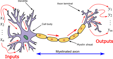
Cell body (Soma): The body of the neuron cell contains the nucleus and carries out biochemical transformation necessary to the life of neurons.
Dendrites: Each neuron has fine, hair-like tubular structures (extensions) around it. They branch out into a tree around the cell body. They accept incoming signals.
Axon: It is a long, thin, tubular structure that works like a transmission line.
Synapse: Neurons are connected to one another in a complex spatial arrangement. When axon reaches its final destination it branches again called terminal arborization. At the end of the axon are highly complex and specialized structures called synapses. The connection between two neurons takes place at these synapses.
Dendrites receive input through the synapses of other neurons. The soma processes these incoming signals over time and converts that processed value into an output, which is sent out to other neurons through the axon and the synapses.
The following diagram represents the general model of ANN which is inspired by a biological neuron. It is also called Perceptron.
A single layer neural network is called a Perceptron. It gives a single output.
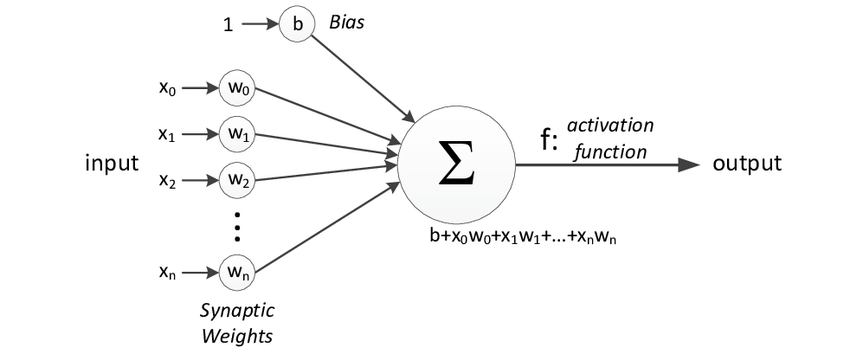
In the above figure, for one single observation, x0, x1, x2, x3...x(n) represents various inputs(independent variables) to the network. Each of these inputs is multiplied by a connection weight or synapse. The weights are represented as w0, w1, w2, w3….w(n). Weight shows the strength of a particular node.
b is a bias value. A bias value allows you to shift the activation function up or down.
In the simplest case, these products are summed, fed to a transfer function (activation function) to generate a result, and this result is sent as output.
Mathematically, x1.w1 + x2.w2 + x3.w3 ...... xn.wn = ∑ xi.wi
Now activation function is applied ????(∑ xi.wi)
Activation function
The Activation function is important for an ANN to learn and make sense of something really complicated. Their main purpose is to convert an input signal of a node in an ANN to an output signal. This output signal is used as input to the next layer in the stack.
Activation function decides whether a neuron should be activated or not by calculating the weighted sum and further adding bias to it. The motive is to introduce non-linearity into the output of a neuron.
If we do not apply activation function then the output signal would be simply linear function(one-degree polynomial). Now, a linear function is easy to solve but they are limited in their complexity, have less power. Without activation function, our model cannot learn and model complicated data such as images, videos, audio, speech, etc.
Now the question arises why do we need Non-Linearity?
Non-Linear functions are those which have a degree more than one and they have a curvature. Now we need a neural network to learn and represent almost anything and any arbitrary complex function that maps an input to output.
Neural Network is considered “Universal Function Approximators”. It means they can learn and compute any function at all.
Types of Activation Functions:
1.Threshold Activation Function — (Binary step function)
A Binary step function is a threshold-based activation function. If the input value is above or below a certain threshold, the neuron is activated and sends exactly the same signal to the next layer.
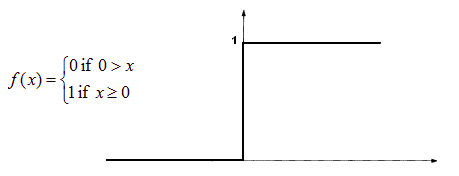
Activation function A = “activated” if Y > threshold
else not or A=1 if y>threshold 0 otherwise.
The problem with this function is for creating a binary classifier ( 1 or 0), but if you want multiple such neurons to be connected to bring in more classes, Class1, Class2, Class3, etc. In this case, all neurons will give 1, so we cannot decide.
2. Sigmoid Activation Function — (Logistic function)
A Sigmoid function is a mathematical function having a characteristic “S”-shaped curve or sigmoid curve which ranges between 0 and 1, therefore it is used for models where we need to predict the probability as an output.
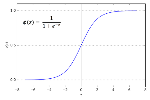
The Sigmoid function is differentiable, means we can find the slope of the curve at any 2 points.
The drawback of the Sigmoid activation function is that it can cause the neural network to get stuck at training time if strong negative input is provided.
3. Hyperbolic Tangent Function — (tanh)
It is similar to Sigmoid but better in performance. It is nonlinear in nature, so great we can stack layers. The function ranges between (-1,1).

The main advantage of this function is that strong negative inputs will be mapped to negative output and only zero-valued inputs are mapped to near-zero outputs.,So less likely to get stuck during training.
4. Rectified Linear Units — (ReLu)
ReLu is the most used activation function in CNN and ANN which ranges from zero to infinity.[0,∞)

It gives an output ‘x’ if x is positive and 0 otherwise. It looks like having the same problem of linear function as it is linear in the positive axis. Relu is non-linear in nature and a combination of ReLu is also non-linear. In fact, it is a good approximator and any function can be approximated with a combination of Relu.
ReLu is 6 times improved over hyperbolic tangent function.
It should only be applied to hidden layers of a neural network. So, for the output layer use softmax function for classification problem and for regression problem use a Linear function.
Here one problem is some gradients are fragile during training and can die. It causes a weight update which will make it never activate on any data point again. Basically ReLu could result in dead neurons.
To fix the problem of dying neurons, Leaky ReLu was introduced. So, Leaky ReLu introduces a small slope to keep the updates alive. Leaky ReLu ranges from -∞ to +∞.
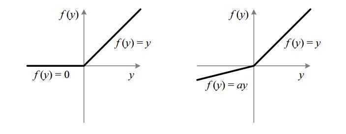
Leak helps to increase the range of the ReLu function. Usually, the value of a = 0.01 or so.
When a is not 0.01, then it is called Randomized ReLu.
How does the Neural network work?
Let us take the example of the price of a property and to start with we have different factors assembled in a single row of data: Area, Bedrooms, Distance to city and Age.
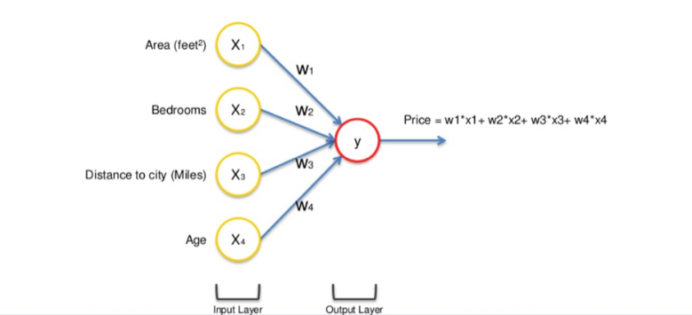
The input values go through the weighted synapses straight over to the output layer. All four will be analyzed, an activation function will be applied, and the results will be produced.
This is simple enough but there is a way to amplify the power of the Neural Network and increase its accuracy by the addition of a hidden layer that sits between the input and output layers.
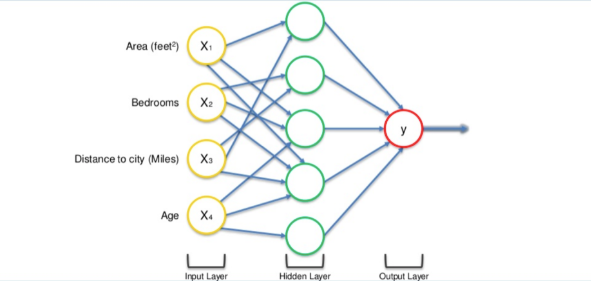
Now in the above figure, all 4 variables are connected to neurons via a synapse. However, not all of the synapses are weighted. they will either have a 0 value or non-0 value.
here, the non-0 value → indicates the importance
0 value → They will be discarded.
Let's take the example of Area and Distance to City are non-zero for the first neuron, which means they are weighted and matter to the first neuron. The other two variables, Bedrooms and Age aren’t weighted and so are not considered by the first neuron.
You may wonder why that first neuron is only considering two of the four variables. In this case, it is common on the property market that larger homes become cheaper the further they are from the city. That’s a basic fact. So what this neuron may be doing is looking specifically for properties that are large but are not so far from the city.
Now, this is where the power of neural networks comes from. There are many of these neurons, each doing similar calculations with different combinations of these variables.
Once this criterion has been met, the neuron applies the activation function and do its calculations. The next neuron down may have weighted synapses of Distance to the city and, Bedrooms.
This way the neurons work and interact in a very flexible way allowing it to look for specific things and therefore make a comprehensive search for whatever it is trained for.
How do Neural networks learn?
Looking at an analogy may be useful in understanding the mechanisms of a neural network. Learning in a neural network is closely related to how we learn in our regular lives and activities — we perform an action and are either accepted or corrected by a trainer or coach to understand how to get better at a certain task. Similarly, neural networks require a trainer in order to describe what should have been produced as a response to the input. Based on the difference between the actual value and the predicted value, an error value also called Cost Function is computed and sent back through the system.
Cost Function: One half of the squared difference between actual and output value.
For each layer of the network, the cost function is analyzed and used to adjust the threshold and weights for the next input. Our aim is to minimize the cost function. The lower the cost function, the closer the actual value to the predicted value. In this way, the error keeps becoming marginally lesser in each run as the network learns how to analyze values.
We feed the resulting data back through the entire neural network. The weighted synapses connecting input variables to the neuron are the only thing we have control over.
As long as there exists a disparity between the actual value and the predicted value, we need to adjust those wights. Once we tweak them a little and run the neural network again, A new Cost function will be produced, hopefully, smaller than the last.
We need to repeat this process until we scrub the cost function down to as small as possible.
The procedure described above is known as Back-propagation and is applied continuously through a network until the error value is kept at a minimum.
There are basically 2 ways to adjust weights: —
1. Brute-force method
2. Batch-Gradient Descent
Brute-force method
Best suited for the single-layer feed-forward network. Here you take a number of possible weights. In this method, we want to eliminate all the other weights except the one right at the bottom of the U-shaped curve.
Optimal weight can be found using simple elimination techniques. This process of elimination work if you have one weight to optimize. What if you have complex NN with many numbers of weights, then this method fails because of the Curse of Dimensionality.
The alternative approach that we have is called Batch Gradient Descent.
Batch-Gradient Descent
It is a first-order iterative optimization algorithm and its responsibility is to find the minimum cost value(loss) in the process of training the model with different weights or updating weights.
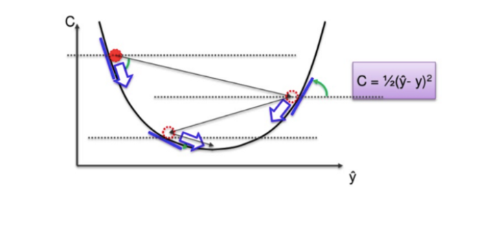
In Gradient Descent, instead of going through every weight one at a time, and ticking every wrong weight off as you go, we instead look at the angle of the function line.
If slope → Negative, that means yo go down the curve.
If slope → Positive, Do nothing
This way a vast number of incorrect weights are eliminated. For instance, if we have 3 million samples, we have to loop through 3 million times. So basically you need to calculate each cost 3 million times.
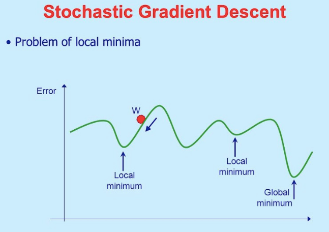
Stochastic Gradient Descent(SGD)
Gradient Descent works fine when we have a convex curve just like in the above figure. But if we don't have a convex curve, Gradient Descent fails.
The word ‘stochastic‘ means a system or a process that is linked with a random probability. Hence, in Stochastic Gradient Descent, a few samples are selected randomly instead of the whole data set for each iteration.
In SGD, we take one row of data at a time, run it through the neural network then adjust the weights. For the second row, we run it, then compare the Cost function and then again adjusting weights. And so on…
SGD helps us to avoid the problem of local minima. It is much faster than Gradient Descent because it is running each row at a time and it doesn’t have to load the whole data in memory for doing computation.
One thing to be noted is that, as SGD is generally noisier than typical Gradient Descent, it usually took a higher number of iterations to reach the minima, because of its randomness in its descent. Even though it requires a higher number of iterations to reach the minima than typical Gradient Descent, it is still computationally much less expensive than typical Gradient Descent. Hence, in most scenarios, SGD is preferred over Batch Gradient Descent for optimizing a learning algorithm.
Training ANN with Stochastic Gradient Descent
Step-1 → Randomly initialize the weights to small numbers close to 0 but not 0.
Step-2 → Input the first observation of your dataset in the input layer, each feature in one node.
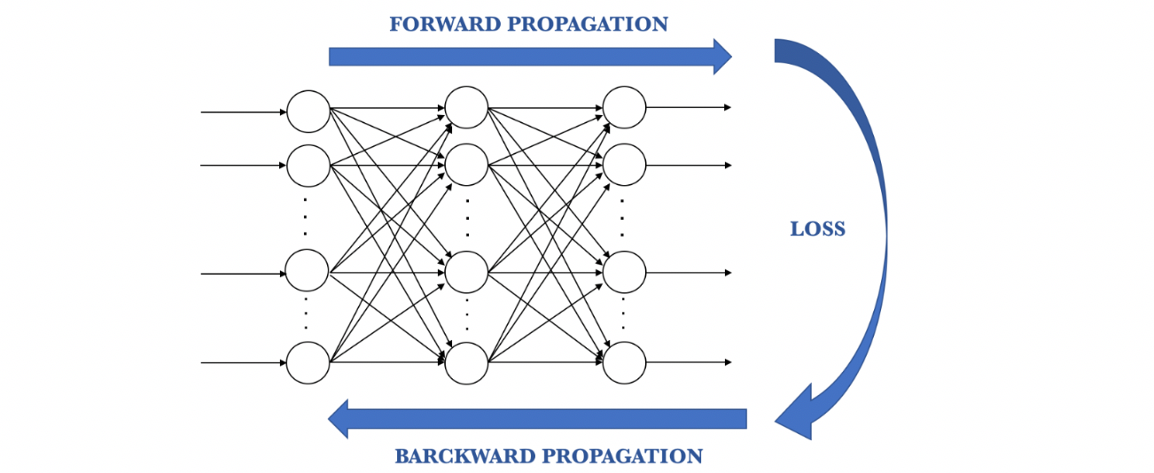
Step-3 → Forward-Propagation: From left to right, the neurons are activated in a way that the impact of each neuron's activation is limited by the weights. Propagate the activations until getting the predicted value.
Step-4 → Compare the predicted result to the actual result and measure the generated error(Cost function).
Step-5 → Back-Propagation: from right to left, the error is backpropagated. Update the weights according to how much they are responsible for the error. The learning rate decides how much we update weights.
Step-6 → Repeat step-1 to 5 and update the weights after each observation(Reinforcement Learning)
Step-7 → When the whole training set passed through the ANN, that makes and epoch. Redo more epochs.
Conclusion
Neural networks are a new concept whose potential we have just scratched the surface of. They may be used for a variety of different concepts and ideas, and learn through a specific mechanism of backpropagation and error correction during the testing phase. By properly minimizing the error, these multi-layered systems may be able to one day learn and conceptualize ideas alone, without human correction.
That's all for this article, In the next article we’ll create an Artificial Neural Network using Keras python library.
I hope you guys have enjoyed reading it. Please share your thoughts/doubts in the comment section. You can reach me out over LinkedIn for any query.
Thanks for reading!!!
Bio: Nagesh Singh Chauhan is a Data Science enthusiast. Interested in Big Data, Python, Machine Learning.
Original. Reposted with permission.
Related:
- A Friendly Introduction to Support Vector Machines
- Introduction to Image Segmentation with K-Means clustering
- Predict Age and Gender Using Convolutional Neural Network and OpenCV