Pro Tips: How to deal with Class Imbalance and Missing Labels
Your spectacularly-performing machine learning model could be subject to the common culprits of class imbalance and missing labels. Learn how to handle these challenges with techniques that remain open areas of new research for addressing real-world machine learning problems.
By Sarfaraz Hussein, Symantec.
“Any AI smart enough to pass a Turing test is smart enough to know to fail it.” - Ian McDonald.
Suppose you are working on a high-impact yet challenging problem of malware classification. You have a large dataset at your disposal and are able to train a machine learning classifier with an accuracy of 98%. While suppressing your excitement, you convince the team to deploy the model, as who would resist a model with such an amazing performance? Quite disappointingly, the model fails to detect threats in the real world!? This unfortunate scenario is all-too-common in classifier development. While there are numerous culprits, one that is common in the security space is the problem of class imbalance. In class imbalance, one trains on a dataset which contains a large number of instances of one type, for example, malicious files, and only a few instances of other types, for example, clean files.

Balancing is never easy. A kitten trying to balance itself on a fence. Credits: Erik Witsoe.
Terminology
Let’s define class imbalance and some terminologies associated with it. We’ll use a simple example of malware classification to make things clear.
Features
Features are the measurable property of the data. They are generally represented as a matrix of dimension number of features x number of dimensions. In the context of malware classification, the features can be opcodes, memory, and file system activities, entropy or learned features through deep learning.
Labels
Labels are class associations that are provided with each feature vector. During training, labels are provided whereas, at test time, labels are predicted. Labels in our example of malware classification are clean and malicious.
Classifier
Classifiers map the features to labels. There are many types of classifiers, but in this article, we’ll think of well-known algorithms like Random Forest, Support Vector Machines and Convolutional Neural Networks. Any of these classifiers can be used to train the malware classification model.
Class Imbalance
As the name implies, class imbalance is a classification challenge in which the proportion of data from each class is not equal. The degree of imbalance can be minor, for example, 4:1, or extreme, like 1000000:1.
Class imbalance is a challenging problem in machine learning, as it may bias the classifier to emphasize the majority class, which can skew the classifier decision boundary and cause overfitting.
Practical Examples of Class Imbalance
Here are a few real-world use cases where class imbalance occurs. Note that a successful classifier for these applications must ultimately overcome class imbalance in order to be effective.
- Spam classification
- Tumor screening in medical data
- Human and car detection for autonomous driving
- Malware classification
- Face recognition
- Fraud detection

Credits: KDNuggets - Drawn by Jon Carter.
Techniques for Overcoming or Addressing Class Imbalance
Now, let’s talk about a few ways to handle class imbalance.
Feature Level Approaches
These approaches change the data distribution by either undersampling the majority classes or oversampling the minority classes so as to balance the data distribution. In undersampling, one can remove instances from the majority class, whereas in oversampling, duplicates of the minority class instances are added to the learning set. Generally, it is advisable to resort to undersampling when you have a large number of training samples and use oversampling when the number of training examples is small.
Both of these two techniques, however, have drawbacks. Undersampling can lead to the loss of useful and potentially discriminative information about the majority class, whereas oversampling cause overfitting. This overfitting while oversampling can be addressed using approaches such as Synthetic Minority Over-sampling Technique (SMOTE) and Adaptive Synthetic Sampling (ADASYN).
In SMOTE, n-neighboring examples around each minority example are sampled, and then on a line connecting these neighboring examples, random points are generated, which serve as the augmented examples. ADASYN, on the other hand, utilizes a weighted distribution of minority class examples based on the local density, thereby inherently accounting for skewed label distribution.
“More data beats clever algorithms, but better data beats more data.” - Peter Norvig
Data Augmentation
Another option to deal with class imbalance is to collect more data. However, in many cases, this option remains exorbitantly expensive in terms of time, effort, and resources. In these cases, data augmentation is a common approach used to add extra samples from the minority class. In the context of images, this is generally achieved by adding distortion to the data by performing translation, rotation, varying the scale as well as by adding different types of noise such as Gaussian, Poisson, and Salt-and-Pepper noise. These transformations to the images can lead to more robust models.
Data augmentation can also provide protection against overfitting along with the dropout and regularization methods. Generally, when label preserving transformations are available (such as in images), it is preferable to use data augmentation over feature level augmentation approaches (such as SMOTE and ADASYN). On the condition of label preservation, the above-mentioned transformation can also be generalized to non-imaging data. Generative Adversarial Networks (GANs) have also been explored for generating augmented training data for a classifier [Bowles et al. 2018].
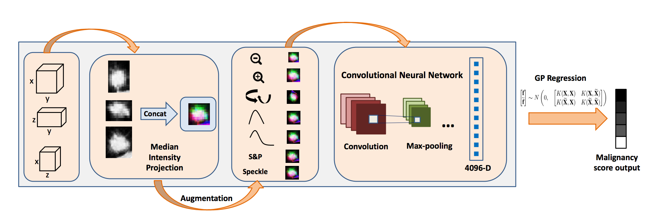
Data augmentation using scaling, rotation and noise for training a deep convolutional network end-to-end used for malignancy determination [Hussein et al. 2017].
Metric Based Approaches
Metric-based approaches change the evaluation criteria used to judge the performance of the classifier. These include the use of accuracy, precision, sensitivity (recall), specificity, ROC, confusion matrices, and other statistics as metrics. For example, in a 95%-5% class imbalance scenario, accuracy cannot be considered as a reliable measure to evaluate a classifier, as it may assign the majority class label of all examples and hence have an accuracy of 95%. In this way, we would be vehemently ignoring the misclassification of minority class, while attributing more significance to the classification of majority class.
Algorithm Level Approaches
Algorithm level approaches actually modify the learning algorithm to improve the performance of the classifier on the minority class. These approaches impose an additional cost for any classification errors pertaining to the minority class and bias the classifier to focus more on the minority class mistakes. Conventionally, cost-sensitive SVM is used as an algorithm level approach to handle class imbalance [Masnadi-Shirazi et al. 2010]:
![]()
where C1 and C2 are the costs for positive and negative slack variables, respectively. Recently, with the popularity of deep learning and convolutional neural networks for classification, there has been increased interest in implicit handling of class imbalance within the network. One way this is implemented is with elastic deformation. Elastic deformations are applied to generate extra samples for training an image segmentation architecture as in U-NET [Ronneberger et al. 2015].
In the computer vision literature, focal loss had been proposed to handle extreme class imbalance between foreground and background for object detection [Lin et al. 2018]. The focal loss goes one step further than handling class imbalance by giving more importance to the hard negatives. It modifies the cross-entropy loss by adding a scalar factor that down-weights the contribution of well-classified examples and focuses more on a sparse set of hard examples. In this manner, it circumvents the detector from being overwhelmed by a large number of easy examples.
Hard-negative mining can be another way of efficiently exploiting the maximum discriminative information from an existing small dataset. These approaches include boot-strapping the classifier by adding false-positives to the negative set in the next training cycle.
Classification with Missing Labels
In addition to class imbalance, the absence of labels is a significant practical problem in machine learning. When only a small number of labeled examples are available, but there is an overall large number of unlabeled examples, the classification problem can be tackled using semi-supervised learning methods. Semi-supervised learning is quite useful for web-page classification, image classification, structural and functional classification of protein, and speech recognition problems.
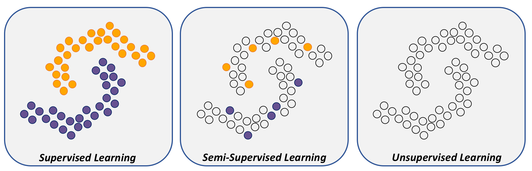
An illustration of training data for supervised, semi-supervised, and unsupervised learning.
There are three popular approaches to address semi-supervised learning problems: (1) self-training, (2) co-training, and (3) graph-based models.
Self-training
In self-training, first, a classifier is trained on the labeled data, and then the learned model is used to make predictions on the unlabeled examples. The high-confidence predictions from the unlabeled samples, along with their predicted labels are appended to the training data, and the model is trained on the new training data. The process is repeated either for a fixed number of iterations or until there are no high-confidence examples left in the unlabeled set. A main drawback of self-training is that high-confidence, but incorrect predictions can be added to the training set, and the mistakes can be amplified in the subsequent training of the model.
Co-training
Co-training requires two feature representations associated with the dataset, which serve as two different views of the data. These representations are dissimilar and conditionally independent, but they can provide complementary information about the data. An example of this situation is phishing website classification, where we can have images and text as two different views of the data.
In co-training, two models are trained separately, one for each representation of the data. During testing, unlabeled samples with highly-confident predictions for exactly one of the models are appended to the training data of the other model. In contrast to self-training, co-training is less susceptible to mistakes from a single model. However, models that use both sets of features are likely to perform better. A generalized form of co-training is multi-view training, where multiple classifiers are trained on different representations of the labeled training data and a majority voting is used to append the unlabeled example to the labeled training data.
Graph-based Approaches
In graph-based approaches, labeled and unlabeled examples are represented as different nodes in a graph where the edges in this graph denote the similarity, or affinity, between adjacent nodes. The assumption in this approach is that nodes with strong edges are likely to share the same label. The affinity function on the edges is computed based on the features of the nodes. The unlabeled nodes in the graph can be labeled using random-walk applied over the graph. In a random-walk approach, an unlabeled node initiates a graph traversal based on the strength of the edges. The walk ends when a labeled node is reached, and a probability that the random walker started at a particular unlabeled node given that it ended at a specific labeled node is computed. In other words, two points are similar if they have indistinguishable starting points. The graph-based semi-supervised learning approach is common for image segmentation problems where each pixel of an image is represented by a node, and a few foreground and background pixels are either manually labeled by the user or assigned labels via image priors.

Machine Learning is simple, eh? Credits: xkcd.com/1838/.
Concluding Remarks
In conclusion, the ways to address these two challenges in machine learning significantly depend on the data as well as the complexity of the problem. In situations where label preserving transformations are available, data-dependent approaches have an upper hand. Recently with deep learning, cost-sensitive training approaches are gaining popularity. Also recently, there has been some interesting work exploring the relationship between transfer learning and semi-supervised learning [Zhou et al. 2018]. Although beyond the scope of this blog, it should be noted that class imbalance is also a practical issue for regression. In summary, class imbalance and missing labels are open research arenas with great potentials of affecting how we address a wide range of real-world machine learning problems.
Original. Reposted with permission.
Bio: Sarfaraz Hussein is a research scientist at the Center for Advanced Machine Learning (CAML) at Symantec, and holds a Ph.D. in Computer Science with a focus on deep learning, computer vision, and medical image analysis.
Related: