Scalable graph machine learning: a mountain we can climb?
Graph machine learning is a developing area of research that brings many complexities. One challenge that both fascinates and infuriates those working with graph algorithms is — scalability. We take a close look at scalability for graph machine learning methods covering what it is, what makes it difficult, and an example of a method that tackles it head-on.
By Kevin Jung, Software Engineer at CSIRO Data61.
Graph machine learning is still a relatively new and developing area of research and brings with it a bucket load of complexities and challenges. One such challenge that both fascinates and infuriates those of us working with graph algorithms is — scalability.
Two methods were positioned early on as the standard approaches to leveraging network information: Graph Convolutional Networks [1] (powerful neural network architecture for machine learning on graphs) and Node2Vec [2] (an algorithmic framework for representational learning on graphs). Both these methods can be very useful for extracting insights from highly-connected datasets.
But I learned first-hand that when trying to apply graph machine learning techniques to identify fraudulent behaviour in the bitcoin blockchain data, scalability was the biggest roadblock. The bitcoin blockchain graph we are using has millions of wallets (nodes) and billions of transactions (edges), which makes most graph machine learning methods infeasible.
In this article, we will take a closer look at scalability for graph machine learning methods: what it is, what makes it difficult, and an example of a method that tries to tackle it head-on.
What is graph machine learning?
First of all, let’s make sure we’re on the same page in terms of what we mean by graph machine learning.
When we say ‘graph,’ we’re talking about a way of representing data as entities with connections between them. In mathematical terms, we call an entity a node or vertex, and a connection an edge. A collection of vertices V, together with a collection of edges E, form a graph G = (V, E).
Graph machine learning is a machine learning technique that can naturally learn and make predictions from graph structured data. We can think of machine learning as a way of learning some transformation function; y = f(x), where x is a piece of data and y is something we want to predict.
Say we take the task of detecting fraudulent bitcoin addresses as an example, and we know the account balance for all addresses on the blockchain. A very simple model might learn to predict that if an address has a zero account balance, then it is unlikely to be fraudulent. In other words, our function f(x) represents a value close to zero (i.e. non-fraudulent) when x is zero:
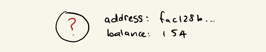
We can agree that simply looking at the account balance of an address is not much to go by when trying to solve such a problem. So at this point, we could consider potential ways to engineer additional features that give our model more information about each address’ behaviour.
What we already have is the rich network structure from the transactions occurring between payers and payees of bitcoin. By designing a model that leverages this information, we’d have more confidence in the results:
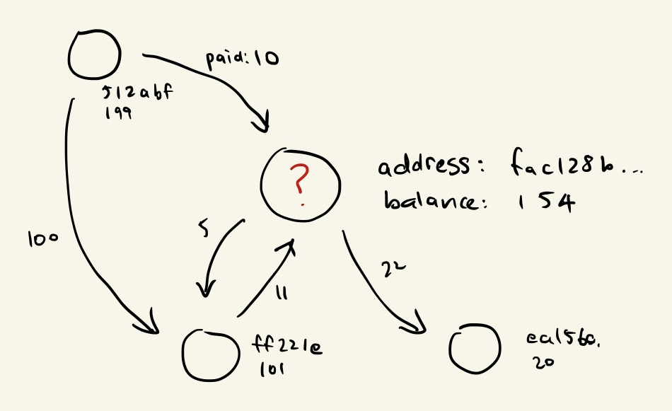
We want to make predictions about addresses not only based on their account balance but also based on transactions made with other addresses. We can try to formulate f such that it is in the form f(x, x’₀, x’₁, …) where x’ᵢ are other data points in the local neighbourhood of x as defined by our graph structure.
One way to achieve this is by making use of graph structure in the form of an adjacency matrix. Multiplying the input data by the adjacency matrix (or some normalisation of) has the effect of linearly combining a data point with its adjacent points.
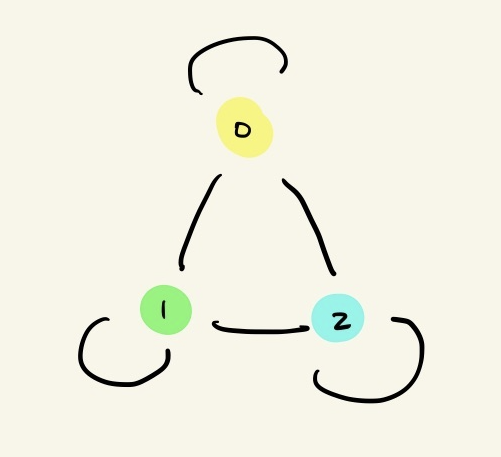
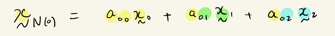
Below is a representation of a graph with three nodes as an adjacency matrix and a set of features:
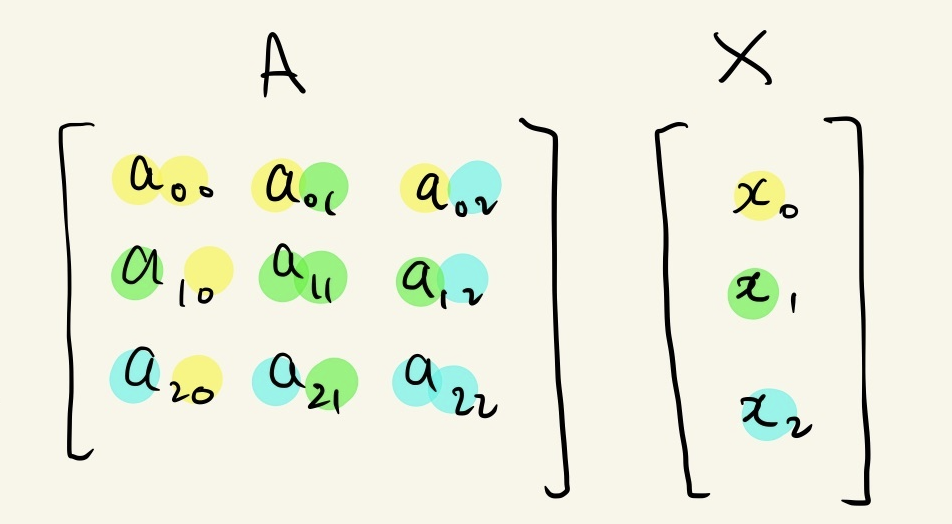
The neighbourhood of node 0 can be aggregated as:
This is the basic high-level principle followed by algorithms like graph convolutional networks. In general, the aggregation of local neighbourhood information is applied recursively to increase the size of the local network that is pulled together to make predictions about a node. (Read StellarGraph’s article Knowing Your Neighbours: Machine Learning on Graphs for a more thorough introduction to these concepts).
What is scalable?
A scalable mountain is a mountain that people can climb. A scalable system is a system that can handle growing demands. A scalable graph machine learning method should be a method that handles growing data sizes… and it also happens to be a huge mountain to climb.
Here, I’m going to argue that the basic principle of naively aggregating across a node’s neighbourhood is not scalable, and describe the problems an algorithm must solve in order to be considered otherwise.
The first problem stems from the fact that one node can be connected arbitrarily to many other nodes from a graph - even the entire graph.
In a more traditional deep learning pipeline, if we want to predict something about x, we only need information about x itself. But with the graph structure in mind, in order to predict something about x we potentially need to aggregate information from the entire dataset. As a dataset gets larger and larger, suddenly we end up aggregating terabytes of data just to make a prediction about a single data point. This doesn’t sound so scalable.
The explanation for the second problem involves understanding the difference between a transductive and an inductive algorithm.
Inductive algorithms try to discover a general rule for the world. The model takes the data as a basis for making predictions for unseen data.
Transductive algorithms attempt to make better predictions for the unlabelled data in a dataset by not generalising a universal model.
When we’re trying to tackle problems in the real world, we’re met with the challenge that the data is not static. Gigabytes of new data may present every day, and this is what makes scalability such an important consideration. But many graph machine learning methods are inherently transductive due to the way information is aggregated from the entire dataset, as opposed to just looking at a single instance of data.
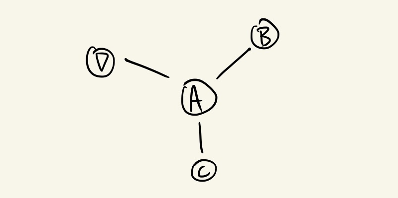
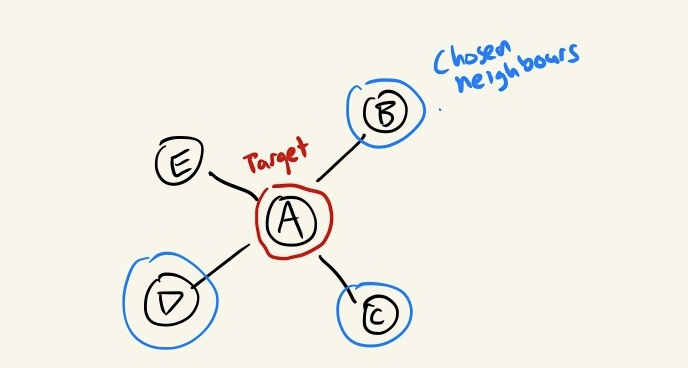
Let’s take a look at a more concrete example that demonstrates this problem. Consider a node A in a graph that is connected to three other nodes B, C, and D:
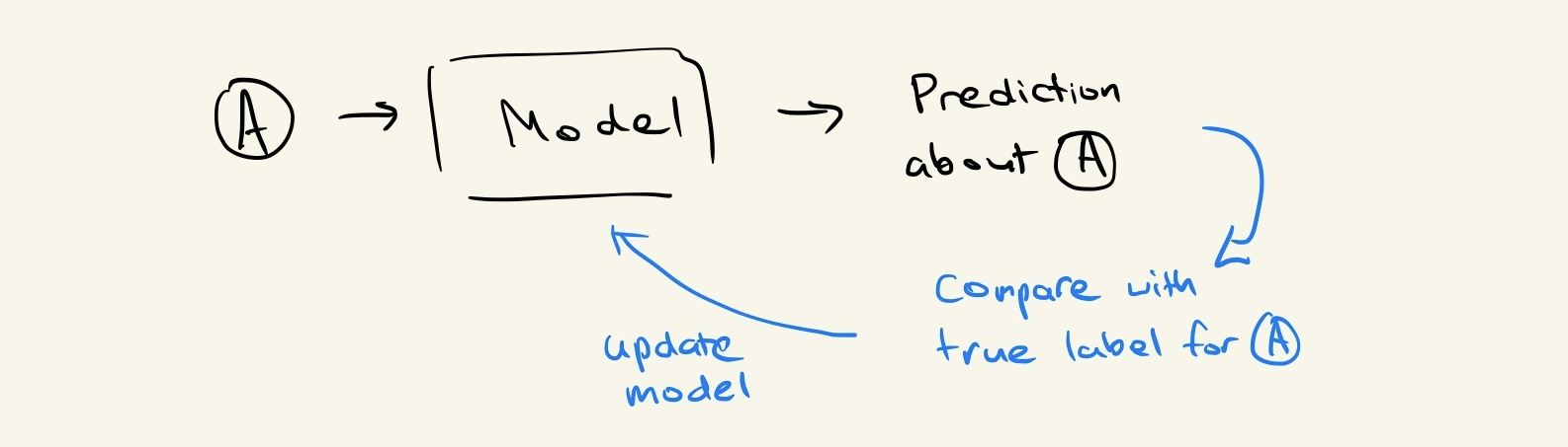
If we weren’t applying any fancy graph methods, we would simply be learning a function that maps from the features of A to a more useful metric; e.g., a prediction we want to make about the node:
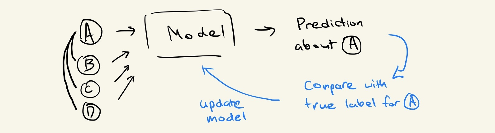
However, as we want to make use of the graph structure, we end up taking the features of B, C, and D as input for the function we’re learning:
Consider that after we’ve trained the model, a new data point arrives some time in the future that happens to be connected to our original node A. We ended up learning a function that doesn’t take this connection into account, so we are stuck in a situation where we’re unsure whether the model we trained is valid for our new set of data.
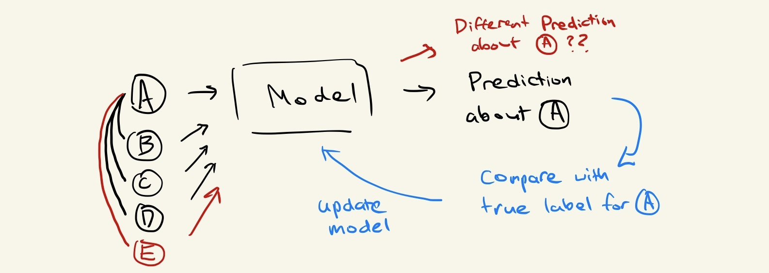
Node E and Edge AE are introduced, causing the Model to also bring in the features of E when aggregating neighbourhood information to make a new prediction for A.
So far, our understanding of graph algorithms suggests they are generally not very scalable, particularly if the algorithm is transductive in nature. Next, we’ll explore an algorithm that attempts to tackle some of these challenges.
Introducing GraphSAGE
A typical way many algorithms try to tackle the scalability problem in graph machine learning is to incorporate some form of sampling. One particular approach we will discuss in this section is the method of neighbour-sampling, which was introduced by the GraphSAGE [3] algorithm.
The SAGE in GraphSAGE stands for Sample-and-Aggregate, which in simple terms means: “for each node, take a sample of nodes from its local neighbourhood, and aggregate their features.”
The concepts of “taking a sample of its neighbours” and “aggregating features” sound rather vague, so let’s explore what they actually mean.
GraphSAGE prescribes that we take a fixed size sample of any given node’s local neighbourhood. This immediately solves our first problem of needing to aggregate information from across the entire dataset. But what are we sacrificing by doing so?
- First and most obviously, taking a sample means we’re taking an approximation of what the neighbourhood actually looks like. Depending on the size of the sample we choose to take, it may be a good enough approximation for our purposes, but an approximation nonetheless.
- We give up the chance for our model to learn something from how connected a node is. For GraphSAGE, a node with five neighbours looks exactly the same as a node with 50 neighbours since we always sample the same number of neighbours for each node.
- Finally, we end up in a world where we could make different predictions about a node based on which neighbours we happened to sample at the time.
Depending on the problem we’d like to solve and what we know about our data, we can try to take a guess at how these issues may affect our results and make a decision about whether GraphSAGE is a suitable algorithm for a particular use-case.
Aggregating features can be done in a number of different ways, but each can be described as a function that takes a list of features from the sampled neighbourhood and outputs an ‘aggregated’ feature vector.
For example, the mean aggregator simply takes the element-wise mean of the features:
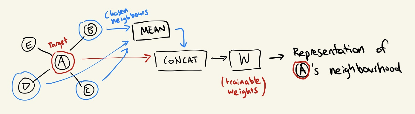
GraphSAGE mean aggregator.
We can then apply a second aggregation step to combine the features of the node itself and its aggregated neighbours. A simple way this can be done, demonstrated above, is to concatenate the two feature vectors and multiply this with a set of trainable weights.
The local sampling nature of GraphSAGE gives us both the inductive algorithm and a mechanism to scale. We are also able to choose the aggregation method to give us some flexibility in the model. Though these benefits come at a cost, where we need to sacrifice model performance for scalability. However, for our purposes, the GraphSAGE algorithm provided a good approach for scaling graph machine learning on the bitcoin dataset.
Success, but not without challenges
GraphSAGE presents the neighbourhood sampling approach to overcome some of the challenges for scalability. Specifically, it:
- gives us a good approximation while bounding the input size for making predictions; and
- allows for an inductive algorithm.
This is a solid breakthrough but doesn’t leave us without problems to be solved.
1. Efficient sampling is still difficult
In order to sample the neighbours of a node without introducing bias, you still need to iterate through all of them. This means although GraphSAGE does restrict the size of the input to the neural network, the step required to populate the input involves looking through the entire graph, which can be very costly.
2. Even with sampling, neighbourhood aggregation still aggregates A LOT of data
Even with a fixed neighbourhood size, applying this scheme recursively means that you get an exponential explosion of the neighbourhood size. For example, if we take 10 random neighbours each time but apply the aggregation over three recursive steps, this ultimately results in a neighbourhood size of 10³.
3. Distributed data introduces even more challenges for graph-based methods
Much of the big data ecosystem revolves around distributing data to enable parallelised workloads and provide the ability to scale out horizontally based on demand. However, naively distributing graph data introduces a significant problem as there is no guarantee that neighbourhood aggregation can be done without communication across the network. This leaves graph-based methods in a place where you pay the cost of shuffling data across the network or miss out on the value of using big data technologies to enable your pipeline.
There are still mountains to climb and more exploration to be done to make scalable graph machine learning more practical. I, for one, will be paying close attention to new developments in this space.
If you’d like to learn more about graph machine learning, feel free to download the open source StellarGraph Python Library or contact us at stellargraph.io.
This work is supported by CSIRO’s Data61, Australia’s leading digital research network.
References
- Graph Convolutional Networks (GCN): Semi-Supervised Classification with Graph Convolutional Networks. Thomas N. Kipf, Max Welling. International Conference on Learning Representations (ICLR), 2017
- Node2Vec: Scalable Feature Learning for Networks. A. Grover, J. Leskovec. ACM SIGKDD International Conference on Knowledge Discovery and Data Mining (KDD), 2016.
- Inductive Representation Learning on Large Graphs. W.L. Hamilton, R. Ying, and J. Leskovec. Neural Information Processing Systems (NIPS), 2017.
Original. Reposted with permission.
Bio: Kevin Jung is a Software Engineer working in the StellarGraph team at CSIRO’s Data61, Australia’s leading digital research network.
Related: