Audio Data Analysis Using Deep Learning with Python (Part 2)

Image Credits

In the previous article, we started our discussion about audio signals; we saw how we can interpret and visualize them using Librosa python library. We also learned how to extract necessary features from a sound/audio file.

We concluded the previous article by building an Artificial Neural Network(ANN) for the music genre classification.

In this article, we are going to build a Convolutional Neural Network for music genre classification.

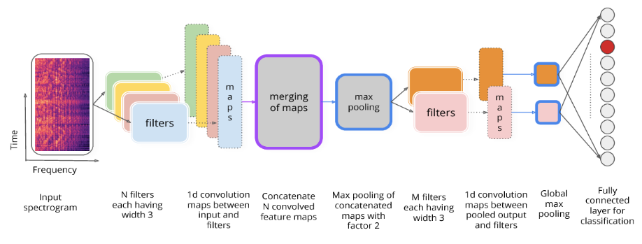
Nowadays, deep learning is more and more used for Music Genre Classification: particularly Convolutional Neural Networks (CNN) taking as entry a spectrogram considered as an image on which are sought different types of structure.

Convolutional Neural Networks (CNN) are very similar to ordinary Neural Networks: they are made up of neurons that have learnable weights and biases. Each neuron receives some inputs, performs a dot product and optionally follows it with a non-linearity. The whole network still expresses a single differentiable score function: from the raw image pixels on one end to class scores at the other. And they still have a loss function (e.g. SVM/Softmax) on the last (fully-connected) layer and all the tips/tricks we developed for learning regular Neural Networks still apply.

So what changes? ConvNet architectures make the explicit assumption that the inputs are images, which allows us to encode certain properties into the architecture. These then make the forward function more efficient to implement and vastly reduce the number of parameters in the network.

Source

They are capable of detecting primary features, which are then combined by subsequent layers of the CNN architecture, resulting in the detection of higher-order complex and relevant novel features.

The dataset consists of 1000 audio tracks each 30 seconds long. It contains 10 genres, each represented by 100 tracks. The tracks are all 22050 Hz monophonic 16-bit audio files in .wav format.

The dataset can be download from marsyas website.

It consists of 10 genres i.e

• Blues
• Classical
• Country
• Disco
• Hiphop
• Jazz
• Metal
• Pop
• Reggae
• Rock

Each genre contains 100 songs. Total dataset: 1000 songs.

Before moving ahead, I would recommend using Google Colab for doing everything related to Neural networks because it is free and provides GPUs and TPUs as runtime environments.

Convolutional Neural Network implementation

Steps involved in extracting features from an input spectrogram and loading it to a fully connected layer.

So let us start building a CNN for genre classification.

To start with load all the required libraries.

import pandas as pd
import numpy as np
from numpy import argmax
import matplotlib.pyplot as plt
%matplotlib inline
import librosa
import librosa.display
import IPython.display
import random
import warnings
import os
from PIL import Image
import pathlib
import csv
# sklearn Preprocessing
from sklearn.model_selection import train_test_split
#Keras
import keras
import warnings
warnings.filterwarnings('ignore')
from keras import layers
from keras.layers import Activation, Dense, Dropout, Conv2D, Flatten, MaxPooling2D, GlobalMaxPooling2D, GlobalAveragePooling1D, AveragePooling2D, Input, Add
from keras.models import Sequential
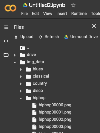
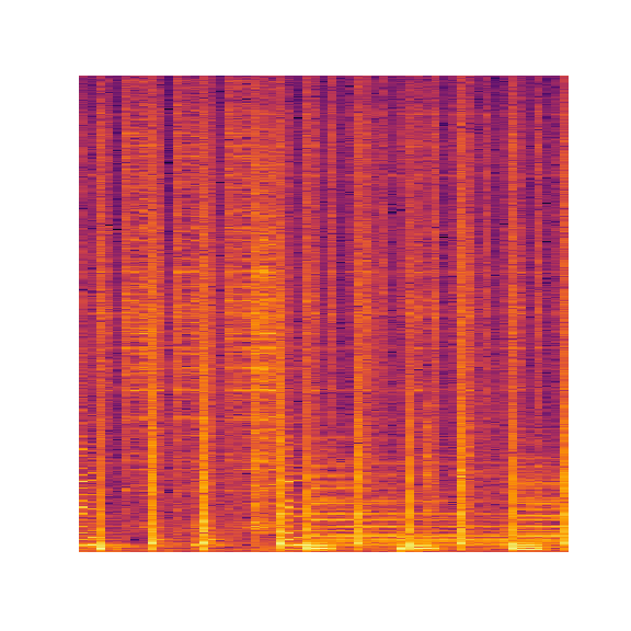
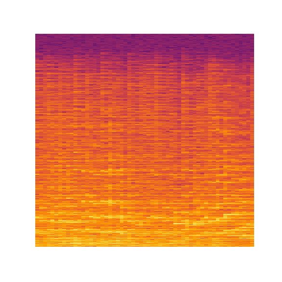
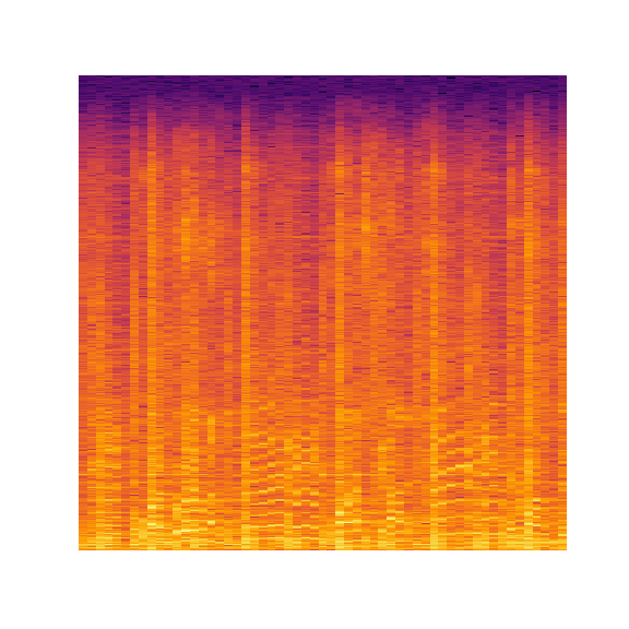
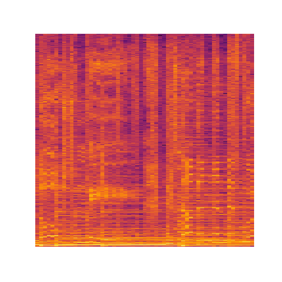
from keras.optimizers import SGD

Now convert the audio data files into PNG format images or basically extracting the Spectrogram for every Audio. We will use librosa python library to extract Spectrogram for every audio file.

genres = 'blues classical country disco hiphop jazz metal pop reggae rock'.split()
for g in genres:
    pathlib.Path(f'img_data/{g}').mkdir(parents=True, exist_ok=True)
    for filename in os.listdir(f'./drive/My Drive/genres/{g}'):
        songname = f'./drive/My Drive/genres/{g}/{filename}'
        y, sr = librosa.load(songname, mono=True, duration=5)
        print(y.shape)
        plt.specgram(y, NFFT=2048, Fs=2, Fc=0, noverlap=128, cmap=cmap, sides='default', mode='default', scale='dB');
        plt.axis('off');
        plt.savefig(f'img_data/{g}/{filename[:-3].replace(".", "")}.png')
        plt.clf()

The above code will create a directory img_data containing all the images categorized in the genre.

Sample spectrograms of Disco, Classical, Blues and Country genre respectively.

   

Disco and Classical

   

Blues and Country

Our next step is to split the data into the train set and test set.

Install split-folders.

pip install split-folders

We will split data by 80% in training and 20% in the test set.

import split-folders
# To only split into training and validation set, set a tuple to `ratio`, i.e, `(.8, .2)`.
split-folders.ratio('./img_data/', output="./data", seed=1337, ratio=(.8, .2)) # default values

The above code returns 2 directories for train and test set inside a parent directory.

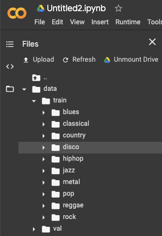
Image Augmentation:

Image Augmentation artificially creates training images through different ways of processing or combination of multiple processing, such as random rotation, shifts, shear and flips, etc.

Perform Image Augmentation instead of training your model with lots of images we can train our model with fewer images and training the model with different angles and modifying the images.

Image Augmentation

Keras has this ImageDataGenerator class which allows the users to perform image augmentation on the fly in a very easy way. You can read about that in Keras’s official documentation.

from keras.preprocessing.image import ImageDataGenerator
train_datagen = ImageDataGenerator(
        rescale=1./255, # rescale all pixel values from 0-255, so aftre this step all our pixel values are in range (0,1)
        shear_range=0.2, #to apply some random tranfromations
        zoom_range=0.2, #to apply zoom
        horizontal_flip=True) # image will be flipper horiztest_datagen = ImageDataGenerator(rescale=1./255)

The ImageDataGenerator class has three methods flow(), flow_from_directory() and flow_from_dataframe() to read the images from a big numpy array and folders containing images.

We will discuss only flow_from_directory() in this blog post.

training_set = train_datagen.flow_from_directory(
        './data/train',
        target_size=(64, 64),
        batch_size=32,
        class_mode='categorical',
        shuffle = False)test_set = test_datagen.flow_from_directory(
        './data/val',
        target_size=(64, 64),
        batch_size=32,
        class_mode='categorical',
        shuffle = False )

flow_from_directory() has the following arguments.

• directory: path where there exists a folder, under which all the test images are present. For example, in this case, the training images are found in ./data/train
• batch_size: Set this to some number that divides your total number of images in your test set exactly.
  Why this only for test_generator?
  Actually, you should set the “batch_size” in both train and valid generators to some number that divides your total number of images in your train set and valid respectively, but this doesn’t matter before because even if batch_size doesn’t match the number of samples in the train or valid sets and some images gets missed out every time we yield the images from generator, it would be sampled the very next epoch you train.
  But for the test set, you should sample the images exactly once, no less or no more. If Confusing, just set it to 1(but maybe a little bit slower).

• class_mode: Set “binary” if you have only two classes to predict, if not set to“categorical”, in case if you’re developing an Autoencoder system, both input and the output would probably be the same image, for this case set to “input”.
• shuffle: Set this to False, because you need to yield the images in “order”, to predict the outputs and match them with their unique ids or filenames.

Create a Convolutional Neural Network:

model = Sequential()
input_shape=(64, 64, 3)#1st hidden layer
model.add(Conv2D(32, (3, 3), strides=(2, 2), input_shape=input_shape))
model.add(AveragePooling2D((2, 2), strides=(2,2)))
model.add(Activation('relu'))#2nd hidden layer
model.add(Conv2D(64, (3, 3), padding="same"))
model.add(AveragePooling2D((2, 2), strides=(2,2)))
model.add(Activation('relu'))#3rd hidden layer
model.add(Conv2D(64, (3, 3), padding="same"))
model.add(AveragePooling2D((2, 2), strides=(2,2)))
model.add(Activation('relu'))#Flatten
model.add(Flatten())
model.add(Dropout(rate=0.5))#Add fully connected layer.
model.add(Dense(64))
model.add(Activation('relu'))
model.add(Dropout(rate=0.5))#Output layer
model.add(Dense(10))
model.add(Activation('softmax'))model.summary()

Compile/train the network using Stochastic Gradient Descent(SGD). Gradient Descent works fine when we have a convex curve. But if we don’t have a convex curve, Gradient Descent fails. Hence, in Stochastic Gradient Descent, few samples are selected randomly instead of the whole data set for each iteration.

epochs = 200
batch_size = 8
learning_rate = 0.01
decay_rate = learning_rate / epochs
momentum = 0.9
sgd = SGD(lr=learning_rate, momentum=momentum, decay=decay_rate, nesterov=False)
model.compile(optimizer="sgd", loss="categorical_crossentropy", metrics=['accuracy'])

Now fit the model with 50 epochs.

model.fit_generator(
        training_set,
        steps_per_epoch=100,
        epochs=50,
        validation_data=test_set,
        validation_steps=200)

Now since the CNN model is trained, let us evaluate it. evaluate_generator() uses both your test input and output. It first predicts output using training input and then evaluates the performance by comparing it against your test output. So it gives out a measure of performance, i.e. accuracy in your case.

#Model Evaluation
model.evaluate_generator(generator=test_set, steps=50)#OUTPUT
[1.704445120342617, 0.33798882681564246]

So the loss is 1.70 and Accuracy is 33.7%.

At last, let your model make some predictions on the test data set. You need to reset the test_set before whenever you call the predict_generator. This is important, if you forget to reset the test_set you will get outputs in a weird order.

test_set.reset()
pred = model.predict_generator(test_set, steps=50, verbose=1)

As of now predicted_class_indices has the predicted labels, but you can’t simply tell what the predictions are, because all you can see is numbers like 0,1,4,1,0,6… You need to map the predicted labels with their unique ids such as filenames to find out what you predicted for which image.

predicted_class_indices=np.argmax(pred,axis=1)

labels = (training_set.class_indices)
labels = dict((v,k) for k,v in labels.items())
predictions = [labels[k] for k in predicted_class_indices]
predictions = predictions[:200]
filenames=test_set.filenames

Append filenames and predictions to a single pandas dataframe as two separate columns. But before doing that check the size of both, it should be the same.

print(len(filename, len(predictions)))
# (200, 200)

Finally, save the results to a CSV file.

results=pd.DataFrame({"Filename":filenames,
                      "Predictions":predictions},orient='index')
results.to_csv("prediction_results.csv",index=False)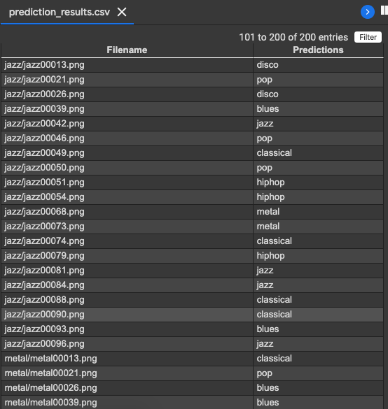

Output

I have trained the model on 50 epochs(which itself took 1.5 hours to execute on Nvidia K80 GPU). If you wanna increase the accuracy, increase the number of epochs to 1000 or even more while training your CNN model.

Conclusion

 
So it shows that CNN is a viable alternative for automatic feature extraction. Such discovery lends support to our hypothesis that the intrinsic characteristics in the variation of musical data are similar to those of image data. Our CNN model is highly scalable but not robust enough to generalized the training result to unseen musical data. This can be overcome with an enlarged dataset and of course the amount of dataset that can be fed.

Well, this concludes the two-article series on Audio Data Analysis Using Deep Learning with Python. I hope you guys have enjoyed reading it, feel free to share your comments/thoughts/feedback in the comment section.

Thanks for reading this article!!!

 
Bio: Nagesh Singh Chauhan is a Big data developer at CirrusLabs. He has over 4 years of working experience in various sectors like Telecom, Analytics, Sales, Data Science having specialisation in various Big data components.

Original. Reposted with permission.

Related:

• Audio File Processing: ECG Audio Using Python
• Basics of Audio File Processing in R
• Artificial Intelligence Books to Read in 2020