Basics of Audio File Processing in R
This post provides basic information on audio processing using R as the programming language. It also walks through and understands some basics of sound and digital audio.
By Taposh Dutta Roy, Kaiser Permanente
In today’s day and age, digital audio has been part and parcel of our life. One can talk to Siri or Alexa or “Ok Google” to search for information. Siri or Alexa or Google knows who is asking for information, and can search for the ask and reply contextually.
The idea of writing this post is to provide basic information on audio processing using R as the programming language. However, before we go to using R as our choice of language, let’s walk through and understand some basics of sound and digital audio.
What is Sound?
Sound is a pressure change of air molecules created by a vibrating object.
This pressure change by vibrating object creates a wave. A wave is how sound propagates. Sound is a thus a mechanical wave that results from the back and forth vibration of the particles of the medium through which the sound wave is moving [4]. Sound is processed through our ears via the ‘auditory’ sense. Thus, sound can also be called as audio. Audio processing a hugely researched domain and lot of very good papers talk about audio processing. As part of this post we will only talk about very basic but helpful information to develop an intuitive understanding.
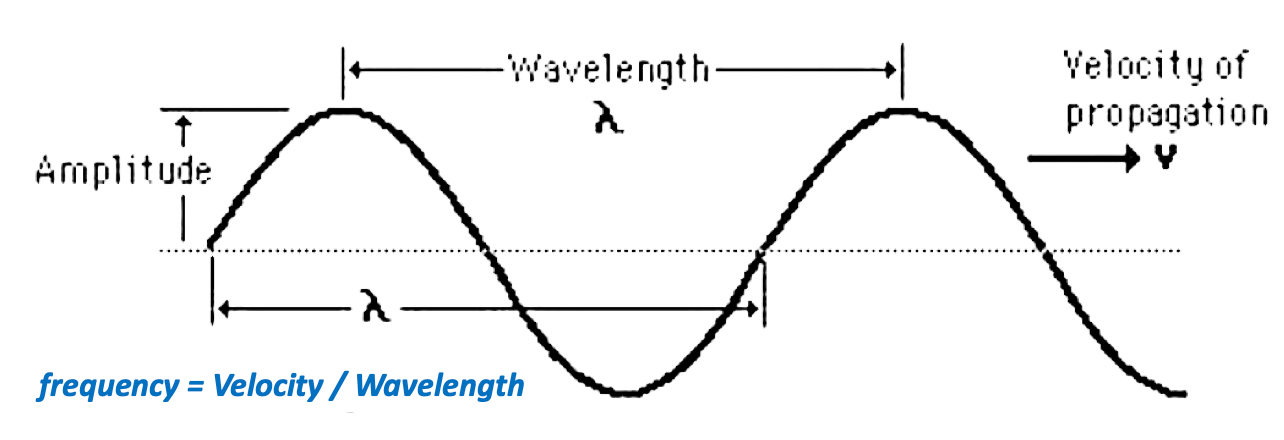
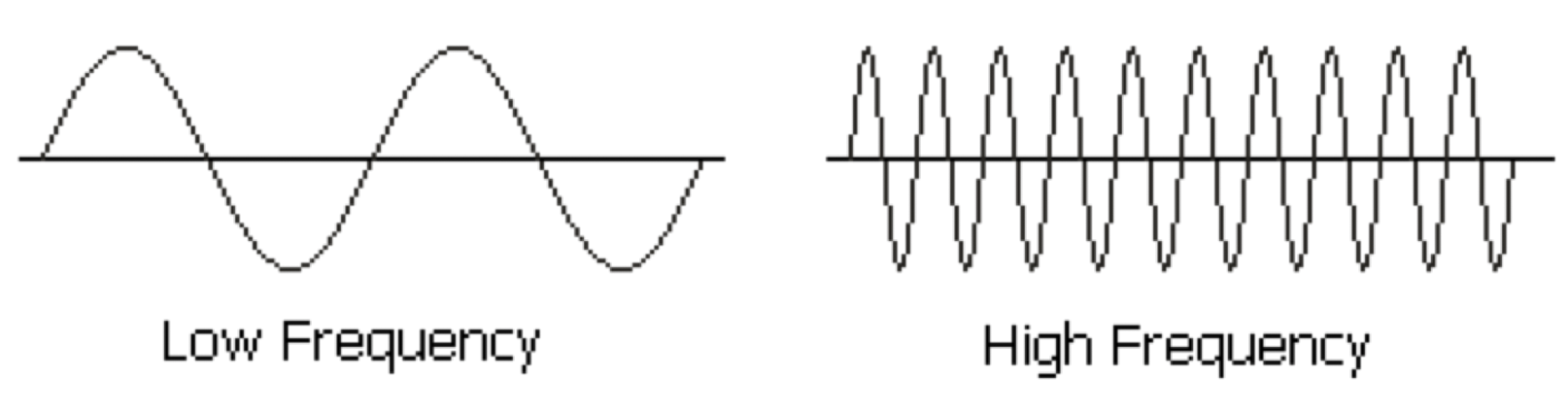
Sound waves can be described by the number of waves per second and the size of the waves. The number of waves per second (or the distance between high or low points) is the frequency of the sound. As shown in the figure above, the horizontal distance between any two successive equivalent points on the wave is called the wavelength. Thus, the wavelength is the horizontal length of one cycle of the wave.
The period of a wave is the time required for one complete cycle of the wave to pass by a point. So, the period is the amount of time it takes for a wave to travel a distance of one wavelength. This understanding is important for analysis of sound as we will move from time domain to frequency domain.
Thus frequency of sound = Velocity of propagation / Wavelength
The size of each wave is described by the amplitude. Amplitude determines how loud or soft a sound will be.
Components of Sound or Audio
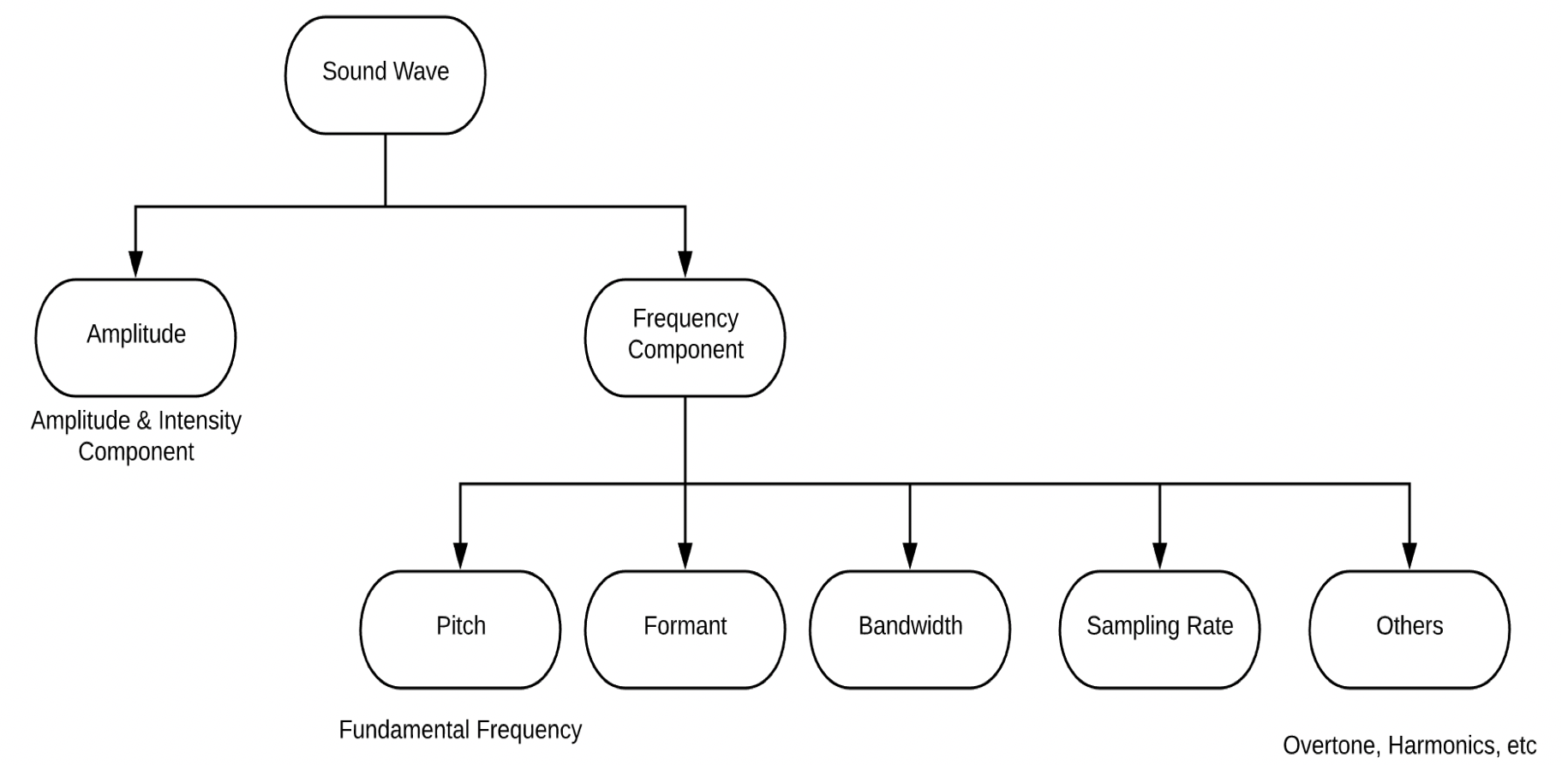
Sound can be divided into multiple components depending on how you want to analyze it. For the purpose of this article, we will classify sound into 2 main components — Amplitude and Frequency. The frequency components can be further divided into — Pitch, Formant, Bandwidth, Sampling Rate, and others (overtone, harmonics etc.)
Amplitude:
As noted, amplitude determines how loud or soft a sound will be. Loudness is a measure of sound wave intensity. Intensity is the amount of energy a sound has over an area. The same sound is more intense if you hear it in a smaller area. In general, we call sounds with a higher intensity louder. Amplitude is a thus a measure of energy. The more energy a wave has, the higher its amplitude. As amplitude increases, intensity also increases.
Some Basic Frequency Components:
Literature provides a variety of frequency components, for the purpose of this article we will talk about the pitch, sampling rate, format, and bandwidth.
Sample rate (or sampling frequency) is the number of samples per second in a Sound. For example: if the sampling rate is 4000 hertz, a recording with a duration of 5 seconds will contain 20,000 samples.
Pitch is the frequency of the fundamental component in the sound, that is, the frequency with which the waveform repeats itself. Pitch depends on the frequency of a sound wave. Frequency is the number of wavelengths that fit into one unit of time.
Formant is a concentration of acoustic energy around a particular frequency in the speech wave. Thus, they are the peaks that are observed in the spectrum envelope.
Bandwidth is the range of frequencies within a given band, in particular that used for transmitting a signal.
Basic Audio Analysis in R
There are a few packages in R which do audio analysis. The key ones that we have seen are : tuneR, wrassp and audio. We use “readr” package to read the wave form.
tuneR Package:
Documentation: https://www.rdocumentation.org/packages/tuneR/versions/1.3.3
Before we go ahead and analyze the entire training data-set, lets analyze a single wave.
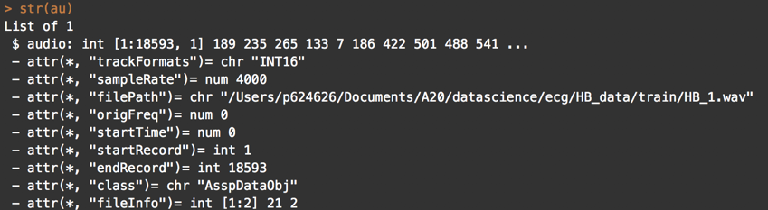
#Read a Wave File
library(readr)
library(tuneR)
#path of file
file_audio_path <- ‘audio_file.wav’
#Read Files
train_audio = readWave(file_audio_path)
#Lets see the structure of the audio.
str(train_audio)
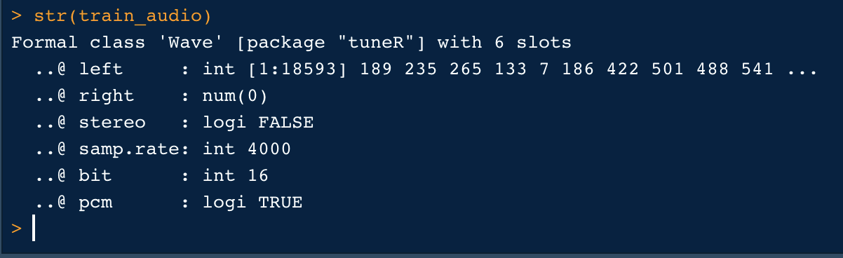
Observations :
The wav file has one channel (@left) containing 18593 sample points each, considering the sample rate (train_audio@samp.rate = 4000) this corresponds to a duration of 4.6s:
18593 /train_audio@samp.rate = 4.6 sec
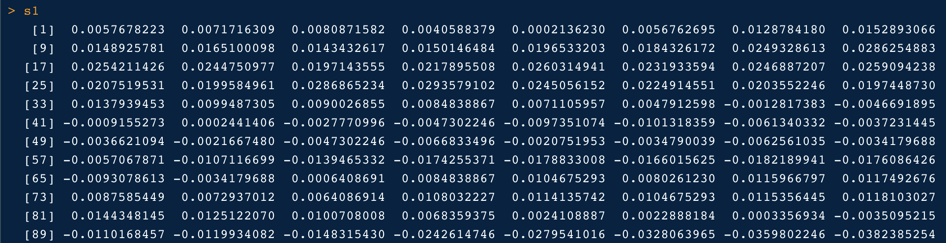
Our wav file has a 16-bit depth (train_audio@bit), this means that the sound pressure values are mapped to integer values that can range from -2¹⁵ to (2¹⁵)-1. We can convert our sound array to floating point values ranging from -1 to 1 as follows:
s1 <- s1 / 2^(train_audio@bit -1)
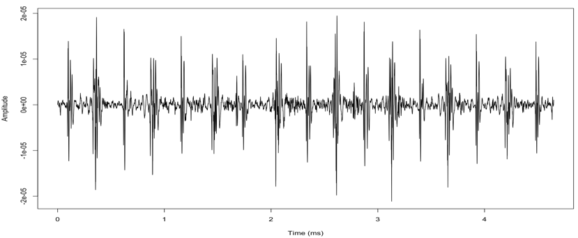
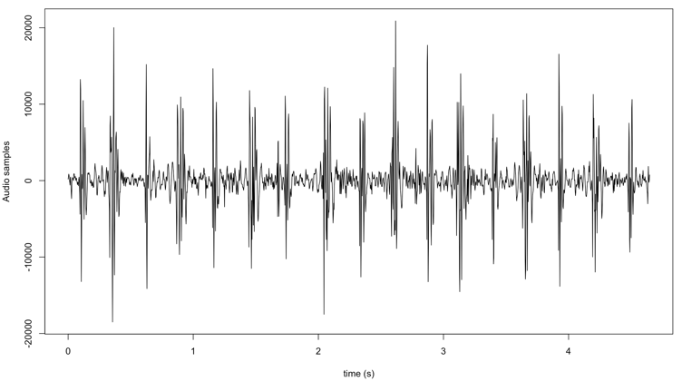
Plotting the Wave:
A time representation of the sound can be obtained by plotting the pressure values against the time axis. However we need to create an array containing the time points first:
timeArray <- (0:(18593–1)) / train_audio@samp.rate
#Plot the wave
plot(timeArray, s1, type=’l’, col=’black’, xlab=’Time (ms)’, ylab=’Amplitude’)
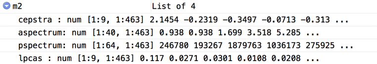
Advanced :
The R-package “tuneR” also provides complex frequency domain analysis functions such as melfcc[8,9,10], audspec etc. There are some good articles that talk about MELFCC such as “The dummy’s guide to MFCC” and “Mel Frequency Cepstral Coefficient (MFCC) tutorial”.
#tuneR
m2 <- melfcc(train_audio, numcep=9, usecmp=TRUE, modelorder=8,
spec_out=TRUE, frames_in_rows=FALSE)
Wrassp Package :
Documentation: https://ips-lmu.github.io/The-EMU-SDMS-Manual/chap-wrassp.html
The package wrassp is capable of more than just the mere reading and writing of specific signal file formats. One can use wrassp to calculate the formant values, their corresponding bandwidths, the fundamental frequency contour and the RMS energy contour of the audio file.
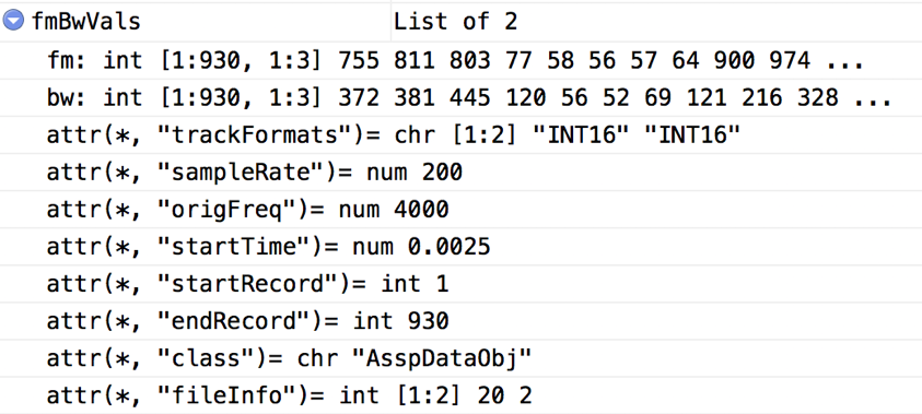
library(wrassp)
# create path to wav file
file_audio_path <- ‘audio_file.wav’
# read audio file
au = read.AsspDataObj(file_audio_path)
str(au)
Observations :
Review the similarities and differences between the output of tuneR package and wrassp. Both provide the same sample rate, number of bits etc. However, wrassp provides a class object AsspDataObj for further use.
# (only plot every 10th element to accelerate plotting)
plot(seq(0,numRecs.AsspDataObj(au) — 1, 10) / rate.AsspDataObj(au),
au$audio[c(TRUE, rep(FALSE,9))],
type=’l’,
xlab=’time (s)’,
ylab=’Audio samples’)
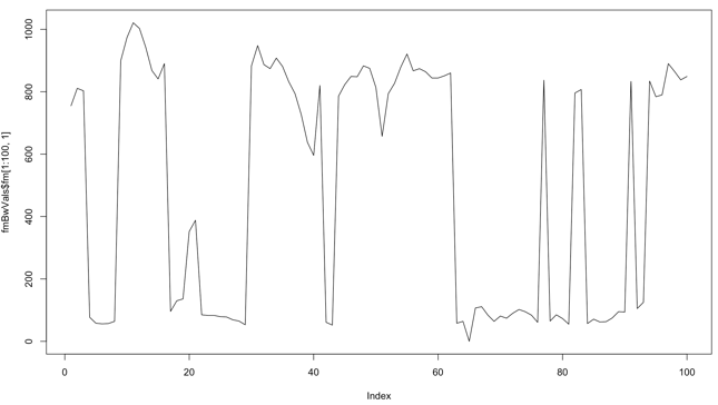
Calculate Formant and Bandwidth :
In the initial part of the tutorial we talked about frequency components — pitch, formant and bandwidth. Let’s compute the formant and bandwidth with wrassp.
# calculate formants and corresponding bandwidth values
fmBwVals = forest(file_audio_path, toFile=F)
fmBwVals
# plot the first 100 F1 values over time:
plot(fmBwVals$fm[1:100,1],type=’l’)
# plot all the formant values
matplot(seq(0,numRecs.AsspDataObj(fmBwVals) — 1) / rate.AsspDataObj(fmBwVals) +
attr(fmBwVals, ‘startTime’),
fmBwVals$fm,
type=’l’,
xlab=’time (s)’,
ylab=’Formant frequency (Hz)’)

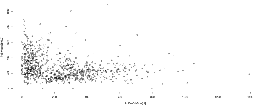
#plot Bandwidth
plot(fmBwVals$bw)
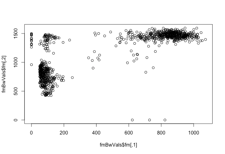
#plot the formant
plot(fmBwVals$fm)
Advanced Functions:
There are a lot of advanced functions that can be explored such as dftSepectrum, RMS energy contour (rmsana), acfana, rfcana etc to add as a feature to your model.
Feature Set Development
Lets use both tuneR and wrassp R-packages and develop an initial set of features for our audio signal.
extract_audio_features <- function(x) {
#tuneR
tr <- readWave(x) # load file
#print(t@left)
ar <- read.AsspDataObj(x)
#File Name
fname <- file_path_sans_ext(basename(x))
#add Feature Number of Samples
num_samples <- numRecs.AsspDataObj(ar)
# calculate formants and corresponding bandwidth values
fmBwVals <- forest(x,toFile=F)
fmVals <- fmBwVals$fm
bwVals <- fmBwVals$bw
#add Feature Sample Rate
sample_rate <- tr@samp.rate
left= tr@left
#left
range_audio = range(tr@left)
#add Feature min_amplitude_range
min_range =range_audio[1]
#add Feature min_amplitude_range
max_range =range_audio[2]
normvalues=left/2^(tr@bit -1)
normal_range <- range(normvalues)
#add Feature normalized_min_amplitude_range
normal_min_ampl_range <- normal_range[1]
#add Feature normalized_min_amplitude_range
normal_max_ampl_range <- normal_range[2]
mylist <- c(fname=fname,num_samples=num_samples,sample_rate=sample_rate, min_range=min_range, max_range=max_range, normal_min_ampl_range=normal_min_ampl_range, normal_max_ampl_range=normal_max_ampl_range,fmVals=fmVals,bwVals=bwVals)
return(as.data.frame(mylist))
}
Now, call this feature extractor function & review
file_audio_path <- ‘../audio_file.wav’
output = extract_audio_features(file_audio_path)
head(output,10)
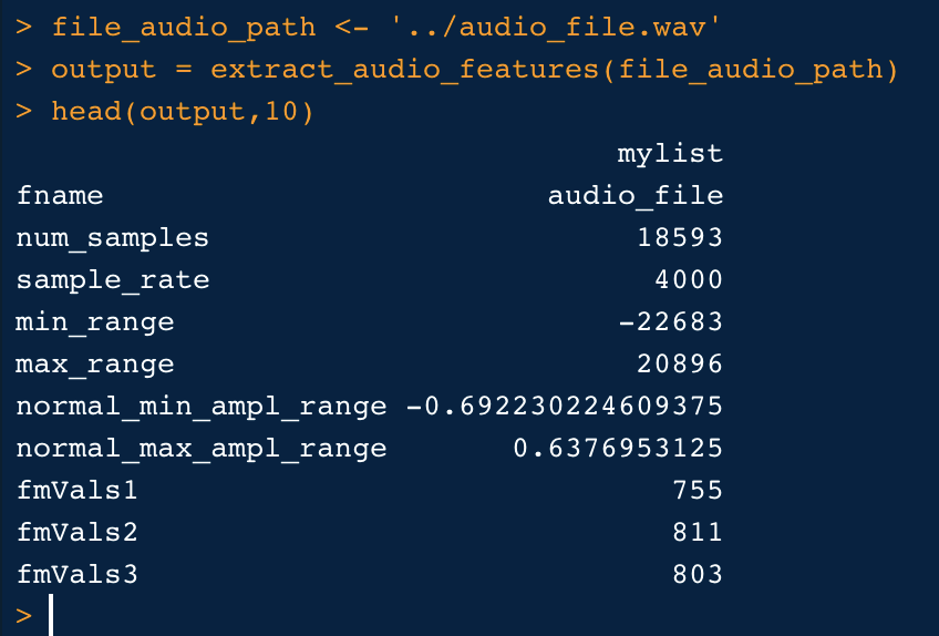
Note, I have used heart beat audio file for this tutorial from kaggle. Finally, use this data for any processing you might need to do. I have shared this code and audio file in my github account. let me know your thoughts.
References
Heartbeat Sounds
Download Open Datasets on 1000s of Projects + Share Projects on One Platform. Explore Popular Topics Like Government…
https://cran.r-project.org/web/packages/seewave/vignettes/seewave_IO.pdf
Individual sound files for each selection (or how to create a warbleR function)
The dummy’s guide to MFCC
Disclaimer 1 : This article is only an introduction to MFCC features and is meant for those in need for an easy and…
http://www.cs.toronto.edu/~gpenn/csc401/soundASR.pdf
https://theproaudiofiles.com/understanding-sound-what-is-sound-part-1
What are the differences between audio and sound?
Answer (1 of 3): In physics, sound (noise, note, din, racket, row, bang, report, hubbub, resonance, reverberation) is a…
Sound as a Mechanical Wave
A sound wave is a mechanical wave that propagates along or through a medium by particle-to-particle interaction. As a…
https://www.nde-ed.org/EducationResources/HighSchool/Sound/components.htm
https://arxiv.org/pdf/1207.5104.pdf
https://www.r-bloggers.com/intro-to-sound-analysis-with-r/
https://medium.com/prathena/the-dummys-guide-to-mfcc-aceab2450fd
https://towardsdatascience.com/getting-to-know-the-mel-spectrogram-31bca3e2d9d0
https://blogs.rstudio.com/tensorflow/posts/2019-02-07-audio-background/
Bio: Taposh Dutta Roy leads Innovation Team of KPInsight at Kaiser Permanente. These are his thoughts based on his personal research. These thoughts and recommendations are not of Kaiser Permanente and Kaiser Permanente is not responsible for the content. If you have questions Mr. Dutta Roy can be reached via LinkedIn.
Original. Reposted with permission.
Related:
- Audio File Processing: ECG Audio Using Python
- How to apply machine learning and deep learning methods to audio analysis
- 10 Python String Processing Tips & Tricks