Recommender System Metrics: Comparing Apples, Oranges and Bananas

By Graydon Snider, Data Scientist at SSENSE

Behind every recommender system lies a bevy of metrics.

 

Introduction

 
Creating a good product recommender system is challenging. Another related challenge, however, is defining what it means to be ‘good’. This article will discuss a sometimes-overlooked aspect of what distinguishes recommender systems from other machine learning tasks: added uncertainties of measuring them.

Let’s imagine that I work for a large grocery store chain that is having a sale on fruit. My task is to make personalized recommendations of three assorted fruits to every customer. Fast forward in time and assume that I have already built a fruit recommender model (yay!), but it is as-yet unproven in practice. Since it’s expensive to run live A/B tests, how might I get some sense of its potential predictive power?

Many models, no matter the complexity, typically involve some form of classification or value estimation: is a transaction fraudulent or not? How much is a customer likely to spend? Discrete predictions are almost always scored via something derived from a confusion matrix, yielding such metrics as precision, recall, Area Under Curve (AUC), and F1 score. For continuous predictive outcomes we get metrics like R-squared, Chi-square, and Mean-Absolute Error (MAE).

 

Ordered Predictions

 
Recommender systems face an additional challenge: order. In our challenge of recommending fruit preferences, suppose I suggest, to a customer named Alice, oranges first and apples second, even though she prefers apples over oranges. Perhaps my recommendations could be improved, but if the order of her preferences is not important, I can then claim (near) perfection. Note that each list does not have to be the same length. Alice might only like three fruits, while we recommend ten.

 

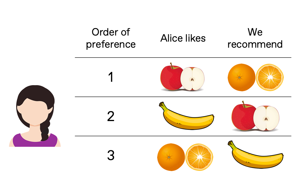
We successfully predicted Alice’s three favorite fruits, but in the wrong order! Should we get a perfect score?

 

How Many Items to Recommend?

 
Here I limited choices to three items, but it’s hard to decide a priori what’s a good number of recommendations. In general the more items we recommend, the less relevant each will likely be, also known as ‘marginal relevance’. We could employ sophisticated practices to decide on a cut-point, or use practical considerations. Consider Google web search results, which technically return everything that’s relevant. But in practice there’s an artificial break between each page that is huge, resulting in a poignant quote:

The Best Place to Hide a Dead Body is Page Two of Google — Anonymous

Despite the many ways to select an optimal list size, here we simply limit ourselves to three fruits per customer. This does not change our goal: we still want to reward the most relevant suggestions in the best order. More value should be awarded to a correct guess near the first position than the last. Luckily, metrics exist to help us out.

 

Scoring Metrics

 
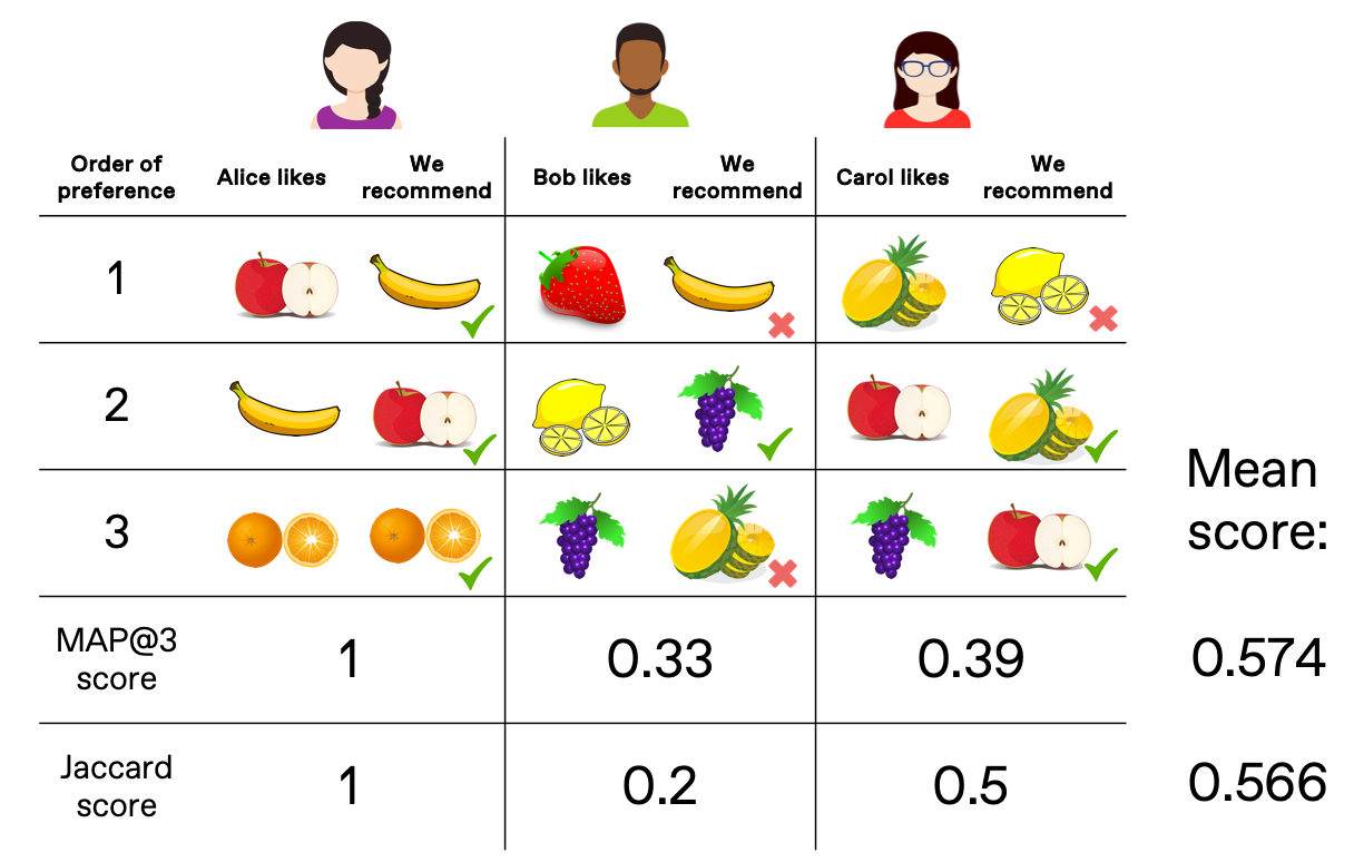
Below are a few examples of three recommended fruits for three customers. How might we score this outcome?

 

Jaccard Index

 
The simplest measure of overlap is the Jaccard Index. In comparing two sets, we calculate the overlap as the number of unique items in both set A and B, then divide by the total number of unique items in the joined sets.

The more items in common, the closer to a perfect score of 1. If no items are in common, the score is zero. For example, Carol’s score is 0.5 because she has two items in common within the ‘recommended’ and ‘true’ sets, then divided by 4 (total number of unique items). But since the Jaccard Index has no sense of order between the two sets up to k items, we turn to another metric: Mean Average Precision.

 

Mean Average Precision at k (MAP@k)

 
We’ll now look at the precision of up to k items. This is calculated by taking an asymmetric approach: preferred (up to k) items remain unordered, but the order of the predicted list matters. The precision score is calculated iteratively moving down through the predicted list.

The scoring for this strategy can seem a little confusing at first (and the name doesn’t help), but it’s more clear when you walk through an example. We gave three recommendations for Carol: lemons, pineapple, and apples. The first recommendation is incorrect since it’s not in her top three favorites, so that gets a precision score of zero. Expanding to two options, one is correct (pineapple) while the other is incorrect (lemons again), yielding a precision score of 1/2. Finally moving to three positions, the precision is 2/3 (two correct guesses out of 3). Combining all three scores gets an average score of 0.39. Rank is implicitly made important because early high precision scores get disproportionately rewarded. Mean average precision is just the scores averaged for multiple people.

 

Other Metrics

 
Generally, MAP@k goes down as k grows. There are other rank metrics, such as Mean Average Recall@k, which increases with k, and Mean Average F1@k, which peaks at some intermediate value of k (hence a way of choosing a non-arbitrary k). We also could decide that order does matter in both the ‘predicted’ and ‘true’ lists, leading to further rewards when matching a user’s top preferences. For example, Normalized Discounted Cumulative Gain (NDCG) is one way to logarithmically regulate the relative importance all the way down an ordered list. NDCG is used in combination with other scoring metrics and quite popular for ranking web searches.

 

Baseline Comparisons

 
Whatever our chosen metric, it is still just a number. What is our relative sense of quality? We need a baseline model to compete against. For example, we could recommend the most popular three fruits to everyone: bananas, apples, and strawberries.

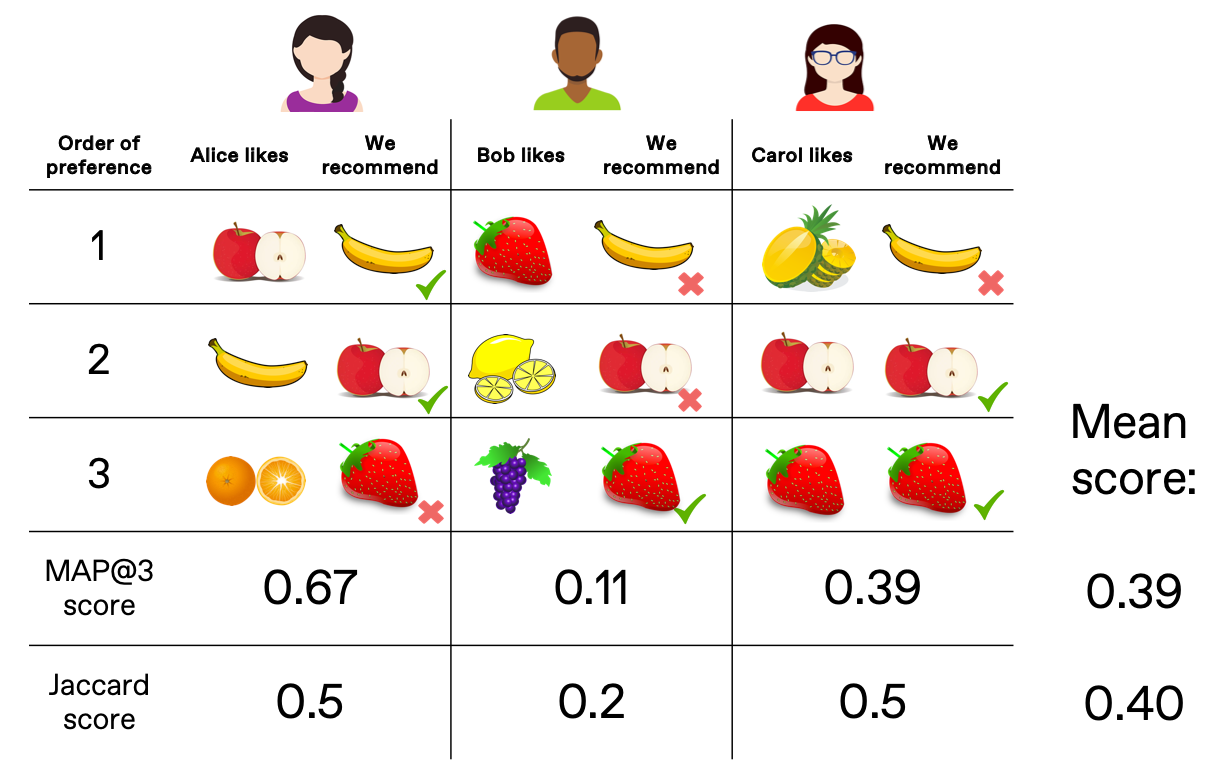
The ‘popular fruits’ scores look good, and it’s no trivial task to outperform them. In fact, a baseline model like this can outperform a more sophisticated model. That’s the bad news. The good news is this very basic model suffers from a lack of diversity, as only three items ever get surfaced. This is bad for net sales as other fruits will never get advertised. We call this metric coverage, and ideally it should be penalized when it’s lacking, although we have not done so here.

The other related drawback of using the baseline in practice is known (appropriately here) as the banana problem, caused when items surface in the recommendation that would have been bought regardless of having been suggested. If an item is popular enough, you may even want to conceal it! A more robust recommender system should have a feedback component, exposing users to some novel suggestions they would not have found on their own (or at least taken longer to discover). Avoiding the banana problem is not explicitly rewarded in our metrics (and really, it should be). This is also very hard to do offline as it deliberately influences user behaviour, which we cannot evaluate in a static data set. Sometimes online A/B tests are the only option.

 

Train / Test Splitting

 
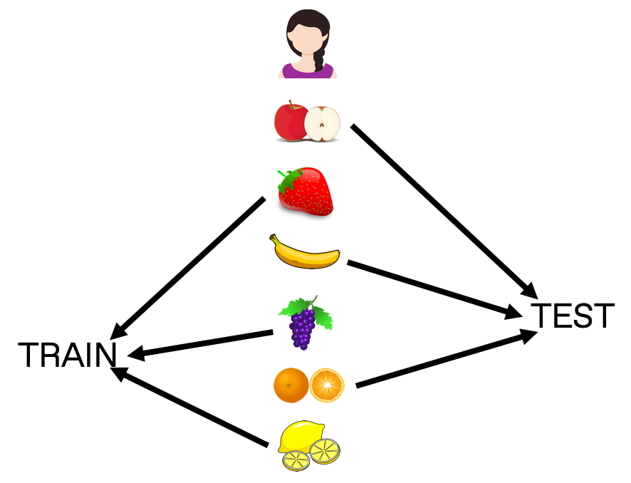
The final topic I wanted to discuss briefly was the question of how to create a train and test set. I have taken for granted that we have ‘true’ and ‘predicted’ ordered sets. But splitting user sets is not trivial. One strategy is to ensure that each customer tested has enough data that some can be withheld in both sets. If Alice, Bob, and Carol had bought six fruits apiece, then I can use three for training, and withhold the other three for testing.

Choosing how to split along the set introduces some additional considerations. For example, this strategy might ignore causality; it is possible training preferences were purchased after the test items unless we introduce a time cut as well. It also might require dropping customers from training with sparse histories, creating a bias towards more frequent shoppers. Training for infrequent purchases such as a house or car may depend entirely on external user profile data. You have to decide what is relevant to your particular situation.

 

Wrapping Up

 
I have provided a brief overview of some challenges faced when evaluating a recommender model offline. These are not completely unique to the subject of recommender systems, but somewhat exaggerated in importance. I would argue that going through each of these steps is worth the mental effort because in designing our metrics, we better understand the problem itself. We can easily create a stream of meaningless evaluation criteria, or create a trivial baseline to surpass, etcetera.

Our definition of success is tied to the k item cutoff point, total item coverage, baseline comparison choice, and even how we split train/test groups. Selecting our objectives can even change the model’s underlying structure, such as hiding suggestions that are already very popular. The final challenge is in choosing the right results to share with stakeholders. Many of these considerations can appear as a distraction, so you must decide carefully what details are helpful to a non-expert to better understand your model. You certainly don’t want to get stuck building a banana-only recommender machine!

Editorial reviews Deanna Chow, Liela Touré, & Prateek Sanyal.

Want to work with us? Click here to see all open positions at SSENSE!

 
Bio: Graydon Snider is a former atmospheric scientist, now a data scientist at SSENSE.

Original. Reposted with permission.

Related:

• Building a Recommender System
• How YouTube is Recommending Your Next Video
• An Easy Introduction to Machine Learning Recommender Systems