Python Pandas For Data Discovery in 7 Simple Steps

When I first started using Python to analyze data, the first line of code that I wrote was ‘import pandas as pd’. I was very confused about what pandas was and struggled a lot with the code. Many questions were in my mind: Why does everyone apply ‘import pandas as pd’ in their first line on Python? What does pandas do that is so valuable?

I believed it would be better if I could have an understanding of its background. Because of my curiosity, I have done some research through different sources, for example; online courses, Google, teachers, etc. Eventually, I got an answer. Let me share that answer with you in this article.

Background

Pandas, the short form from Panel Data, was first released on 11 Jan 2008 by a well-known developer called Wes McKinney. Wes McKinney hated the idea of researchers wasting their time. I eventually understood the importance of pandas from what he said in his interview.

“Scientists unnecessarily dealing with the drudgery of simple data manipulation tasks makes me feel terrible,”

“I tell people that it enables people to analyze and work with data who are not expert computer scientists,”

Pandas is one of the main tools used by data analysts nowadays and has been instrumental in boosting Python’s usage in the data scientist community. Python has been growing rapidly in terms of users over the last decade or so, based on traffic to the StackOverflow question and answer site. The graph below shows the huge growth of Pandas compared to some other Python software libraries!

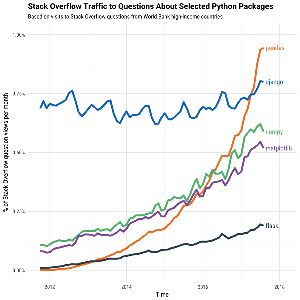
reference: coding club

It’s time to start! Let’s get your hands dirty with some coding! It’s not difficult and is suitable for any beginner. There are 7 steps in total.

Step 1: Importing library

import pandas as pd

Step 2: Reading data

Method 1: load in a text file containing tabular data

df=pd.read_csv(‘clareyan_file.csv’)

Method 2: create a DataFrame in Pandas from a Python dictionary

#create a Python script that converts a Python dictionary{ } into a Pandas DataFrame
df = pd.DataFrame({
    'year_born': [1984, 1998, 1959, pd.np.nan, 1982, 1990, 1989, 1974, pd.np.nan, 1982], 
    'sex': ['M', 'W', 'M', 'W', 'W', 'M', 'W', 'W', 'M', 'W'],
    'name': ['George', 'Elizabeth', 'John', 'Julie', 'Mary', 'Bob', 'Jennifer', 'Patricia', 'Albert', 'Linda']
})
#display the top 5 rows 
df.head()
#display the top 10
df.head(10)
#display the bottom 5 rows
df.tail(5)

Output

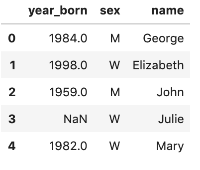
Here, I used: df.head() Remark: python lists are 0-indexed so the first element is 0, second is 1, so on.

Step 3: Understanding the data types, number of rows and columns

df.shape

Output

(10,3) #(row, column)

print('Number of variables: {}'.format(df.shape[1]))
print('Number of rows: {}'.format(df.shape[0]))

Output

Number of variables: 3

Number of rows: 10

The data type is an important concept in programming, it contains classification or categorization of data items.

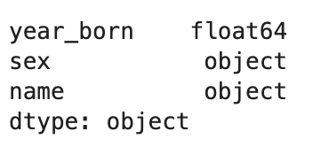
# Check the data type
df.dtypes

Output

If you are not familiar with data types, this table may be useful for you.

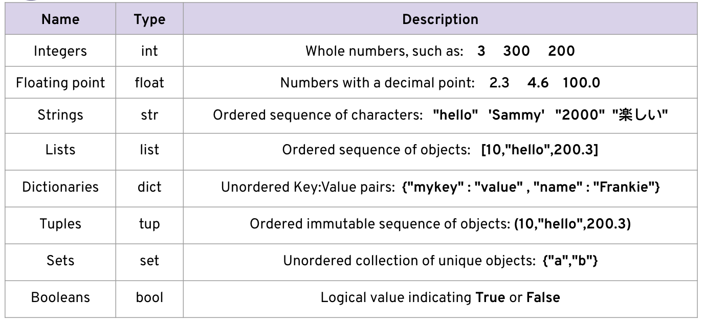
Data Types

# basic data information(columns, rows, data types and memory usage)
df.info()

Output

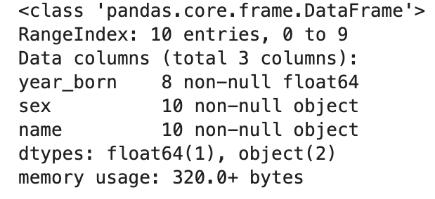
From the output, we know there are 3 columns, taking 153MB of memory.

Step 4: Observing categorical data

#use the dataframe.nunique() function to find the unique values
unique_counts = pd.DataFrame.from_records([(col, df[col].nunique()) for col in df.columns],columns=['Column_Name', 'Num_Unique']).sort_values(by=['Num_Unique'])

Output

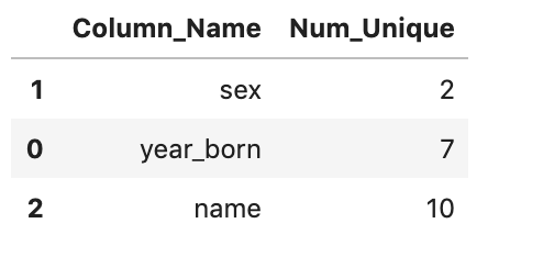
The table above highlights the unique values of each column that could allow you to determine which values may be potentially categorical. For example, the unique number of sex is 2 (which makes sense [M/F]). It is less likely that name and year_born are categorical variables because the number of unique is pretty large.

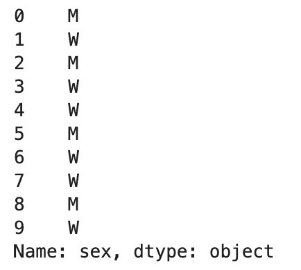
#inspect the categorical column in detail
df['sex']

Output

# Counting
df.sex.value_counts()

Output

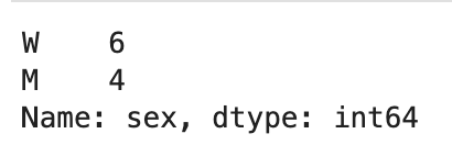
6 females and 4 males

Step 5: Exploring data

# look into the specify data
df[(df['sex']=='M') & (df['year_born']==1990)]

Output

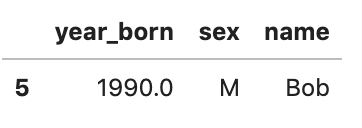
To use & (AND), ~ (NOT) and | (OR), you have to add “(“ and “)” before and after the logical operation.

Besides, with loc and iloc you can do practically any data selection operation on DataFrames you can think of. Let me give you some examples.

#show the row at position zero (1st row)
df.iloc[0]

Output

#show the 1st column and 1st row
df.iloc[0,0]

Output

1984

Next, I’ll use loc to do the data selection.

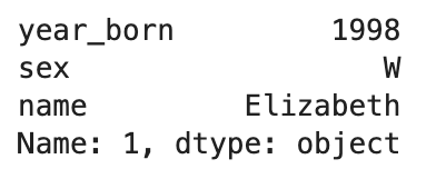
#Gives you the row at position zero (2nd row)
df.loc[1]

Output

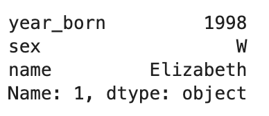
2nd row

#give you the first row and the column of 'sex'
df.loc[0,'sex']

Output

‘M’

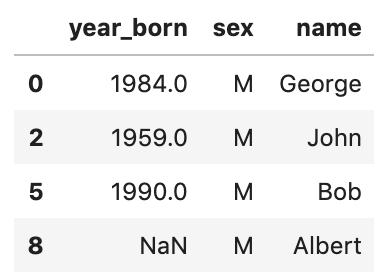
#select all rows where sex is male
df.loc[df.sex=='M']

Output

#only show the column of 'year born' where sex is male
df.loc[df.sex=='M','year_born']

Output

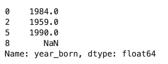
# find the mean of year_born of male
df.loc[df.sex=='M', 'year_born'].median()

Output

1984.0

other aggregations: min(), max(),sum(), mean(), std()

From the above examples, you should know how to use the function of iloc and loc. iloc is short for “integer location”. iloc gives us access to the DataFrame in ‘matrix’ style notation, i.e., [row, column] notation. loc is label-based, which means that you have to specify rows and columns based on their row and column labels (names).

From my experience, people would easily mix up with the usage of loc and iloc. Therefore I would prefer to stick on one — loc.

Step 6: Finding the missing values

#find null values and sort descending
df.isnull().sum().sort_values(ascending=False)

Output

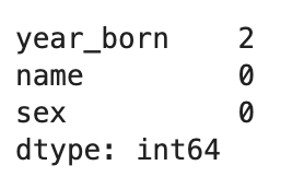
2 missing values in the column of ‘year_born’.

Step 7: Handling missing values

When inplace=True is passed, the data is renamed in place.

#method 1: fill missing value using mean
df['year_born'].fillna((df['year_born'].mean()), inplace= True)

Output

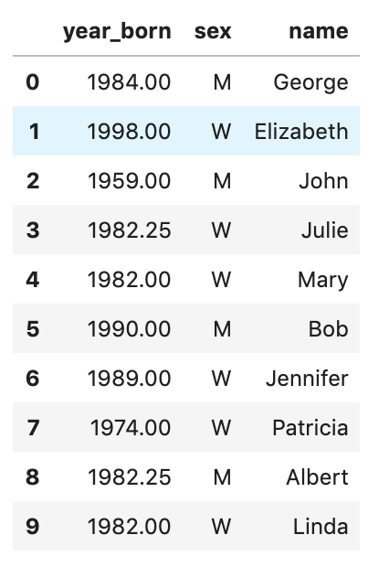
The year_born of Julie and Albert is 1982.25 (replaced by mean).

#method 2 drop the rows with missing value
df.dropna(inplace = True)

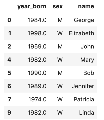
4th and 9th rows are dropped.

Step 8: Visualising data

Matplotlib is a Python 2D plotting library. You can easily generate plots, histograms, power spectra, bar charts, scatterplots, etc., with just a few lines of code. The example here is plotting a histogram. The “%matplotlib inline” will make your plot outputs appear and be stored within the notebook, but it is not related to how pandas.hist() works.

%matplotlib inline
df.loc[df.sex=='W', 'year_born'].hist()

Output

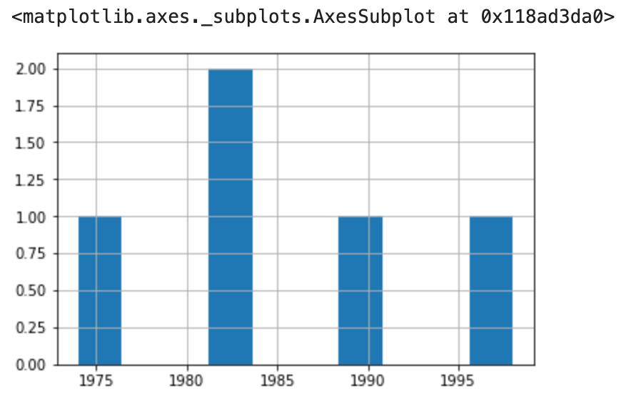
The year_born where sex=’W’.

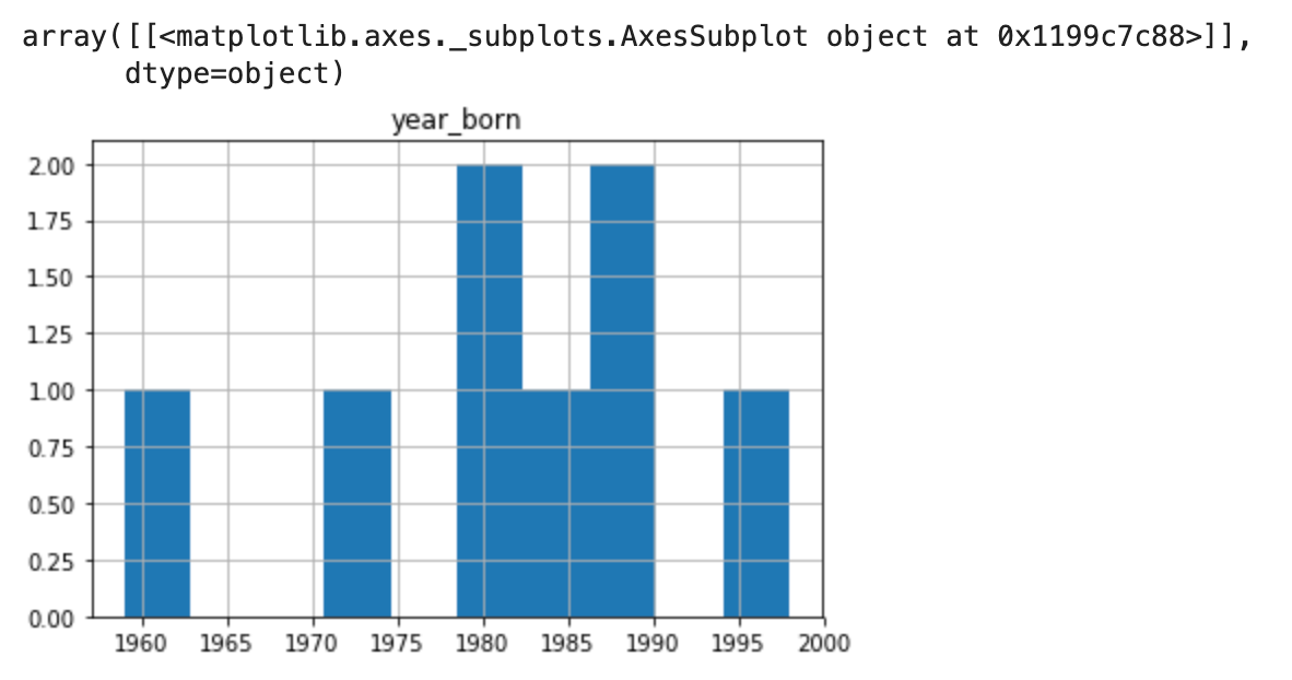
#plot a histogram showing 'year_born'
df.hist(column='year_born')

Output

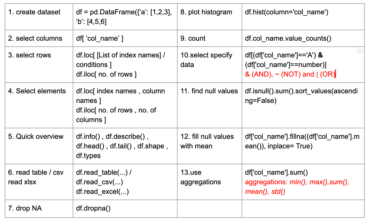
Great! I have already gone through all 7steps on data discovery using pandas library. Let me sum up what functions that I have used:

Bonus: Let me introduce the fastest way to do exploratory data analysis (EDA) with only two lines of code: pandas_profiling

import pandas_profiling
df.profile_report()

It covers:

1. Overview:

Dataset info: Number of variables, Number of observations, Missing cells, Duplicate rows 0, Total size in memory and Average record size in memory

2. Variables: Missing values and its percentage, Distinct count, Unique
3. Correlations
4. Missing Values: ‘Matrix’ and ‘Count’
5. Sample: First 10 rows and Last 10 rows

Original. Reposted with permission.

Related:

• Data Cleaning and Preprocessing for Beginners
• 5 Advanced Features of Pandas and How to Use Them
• How to Speed up Pandas by 4x with one line of code