Sparse Matrix Representation in Python
Leveraging sparse matrix representations for your data when appropriate can spare you memory storage. Have a look at the reasons why, see how to create sparse matrices in with Python, and compare the memory requirements for standard and sparse representations of the same data.
Most machine learning practitioners are accustomed to adopting a matrix representation of their datasets prior to feeding the data into a machine learning algorithm. Matrices are an ideal form for this, usually with rows representing dataset instances and columns representing features.
A sparse matrix is a matrix in which most elements are zeroes. This is in contrast to a dense matrix, the differentiating characteristic of which you can likely figure out at this point without any help.
Often our data is dense, with feature columns filled up for every instance we have. If we are using a finite number of columns to robustly describe some thing, generally the allotted descriptive values for a given data point have their work cut out for them in order to provide meaningful representation: a person, an image, an iris, housing prices, a potential credit risk.
But some types of data are not in need of such verbosity in their representation. Think relationships. There may be a large number of potential things we need to capture the relationship status of, but at the intersection of these things we may need to simply record either yes, there is a relationship, or no, there is not.
Did this person purchase that item? Does that sentence have this word in it? There are a lot of potential words that could show up in any given sentence, but not very many of them actually do. Similarly, there may be a lot of items for sale, but any individual person will not have purchased many of them.
This is one way in which sparse matrices come into play in machine learning. Picture a column as items for sales, and rows as shoppers. For every intersection where a given item was not purchased by a given shopper, there would be a "no" (null) representation, such as a 0. Only intersections where the given item was purchased by a given shopper would there need to be a "yes" representation, such as a 1. The same goes for occurrences of given words in given sentences. You can see why such matrices would contain many zeroes, meaning they would be sparse.
One problem that comes up with sparse matrices is that they can be very taxing on memory. Assuming you take a standard approach to representing a 2x2 matrix, allocations for every null representation need to be made in memory, though there is no useful information captured. This memory taxation continues on to permanent storage as well. In a standard approach to matrix representation, we are forced to also record the absence of a thing, as opposed to simply its presence.
But wait. There's got to be a better way!
It just so happens that there is. Sparse matrices need not be represented in the standard matrix form. There are a number of approaches to relieving the stress that this standard form puts our computational systems under, and it just so happens that some algorithms in prevalent Python machine learning workhorse Scikit-learn accept some of these sparse representations as input. Getting familiar could save you time, trouble, and sanity.
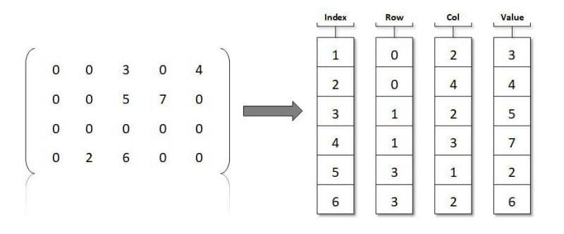
How can we better represent these sparse matrices? We need a manner in which to track where zeroes are not. What about a 2 column table, in which we track in one column the row,col of where a non-zero item exists, and its corresponding value in the other column? Keep in mind there is no necessity for sparse matrices to only house zeroes and ones; so long as most elements are zeroes, the matrix is sparse, regardless of what exists in non-zero elements.
We also need an order in which we go about creating the sparse matrix — do we go row by row, storing each non-zero element as we encounter them, or do we go column by column? If we decide to go row by row, congratulations, you have just created a compressed sparse row matrix. If by column, you now have a compressed sparse column matrix. Conveniently, Scipy includes support for both.
Let's have a look at how to create these matrices. First we create a simple matrix in Numpy.
import numpy as np
from scipy import sparse

X = np.random.uniform(size=(6, 6))
print(X)
[[0.79904211 0.76621075 0.57847599 0.72606798 0.10008544 0.90838851]
 [0.45504345 0.10275931 0.0191763  0.09037216 0.14604688 0.02899529]
 [0.92234613 0.78231698 0.43204239 0.61663291 0.78899765 0.44088739]
 [0.50422356 0.72221353 0.57838041 0.30222171 0.25263237 0.55913311]
 [0.191842   0.07242766 0.17230918 0.31543582 0.90043157 0.8787012 ]
 [0.71360049 0.45130523 0.46687117 0.96148004 0.56777938 0.40780967]]
Then we need to zero out a majority of the matrix elements, making it sparse.
X[X < 0.7] = 0
print(X)
[[0.79904211 0.76621075 0.         0.72606798 0.         0.90838851]
 [0.         0.         0.         0.         0.         0.        ]
 [0.92234613 0.78231698 0.         0.         0.78899765 0.        ]
 [0.         0.72221353 0.         0.         0.         0.        ]
 [0.         0.         0.         0.         0.90043157 0.8787012 ]
 [0.71360049 0.         0.         0.96148004 0.         0.        ]]
Now we store standard matrix X as a compressed sparse row matrix. In order to do so, elements are traversed row by row, left to right, and entered into this compressed matrix representation as they encountered.
X_csr = sparse.csr_matrix(X)
print(X_csr)
  (0, 0)	0.799042106215471
  (0, 1)	0.7662107548809229
  (0, 3)	0.7260679774297479
  (0, 5)	0.9083885095042665
  (2, 0)	0.9223461264672205
  (2, 1)	0.7823169848589594
  (2, 4)	0.7889976504606654
  (3, 1)	0.7222135307432606
  (4, 4)	0.9004315651436953
  (4, 5)	0.8787011979799789
  (5, 0)	0.7136004887949333
  (5, 3)	0.9614800409505844
Presto!
And what about a compressed sparse column matrix? For its creation, elements are traversed column by column, top to bottom, and entered into the compressed representation as they are encountered.
X_csc = sparse.csc_matrix(X)
print(X_csc)
  (0, 0)	0.799042106215471
  (2, 0)	0.9223461264672205
  (5, 0)	0.7136004887949333
  (0, 1)	0.7662107548809229
  (2, 1)	0.7823169848589594
  (3, 1)	0.7222135307432606
  (0, 3)	0.7260679774297479
  (5, 3)	0.9614800409505844
  (2, 4)	0.7889976504606654
  (4, 4)	0.9004315651436953
  (0, 5)	0.9083885095042665
  (4, 5)	0.8787011979799789
Note the differences between the resultant sparse matrix representations, specifically the difference in location of the same element values.
As noted, many Scikit-learn algorithms accept scipy.sparse matrices of shape [num_samples, num_features] is place of Numpy arrays, so there is no pressing requirement to transform them back to standard Numpy representation at this point. There could also be memory constraints preventing one from doing so (recall this was one of the main reasons for employing this approach). However, just for demonstration, here's how to convert a sparse Scipy matrix representation back to a Numpy multidimensional array.
print(X_csr.toarray())
[[0.79904211 0.76621075 0.         0.72606798 0.         0.90838851]
 [0.         0.         0.         0.         0.         0.        ]
 [0.92234613 0.78231698 0.         0.         0.78899765 0.        ]
 [0.         0.72221353 0.         0.         0.         0.        ]
 [0.         0.         0.         0.         0.90043157 0.8787012 ]
 [0.71360049 0.         0.         0.96148004 0.         0.        ]]
And what about the difference in memory requirements between the 2 representations? Let's go through the process again, starting off with a larger matrix in standard Numpy form, and then compute the memory (in bytes) that each representation uses.
import numpy as np
from scipy import sparse

X = np.random.uniform(size=(10000, 10000))
X[X < 0.7] = 0
X_csr = sparse.csr_matrix(X)

print(f"Size in bytes of original matrix: {X.nbytes}")
print(f"Size in bytes of compressed sparse row matrix: {X_csr.data.nbytes + X_csr.indptr.nbytes + X_csr.indices.nbytes}")
Size in bytes of original matrix: 800000000
Size in bytes of compressed sparse row matrix: 360065312
There you can see a significant savings in memory that the compressed matrix form enjoys over the standard Numpy representation, approximately 360 megabytes versus 800 megabytes. That's a 440 megabyte savings, with nearly no time overhead, given that the conversion between formats is highly optimized. Obviously these sparse SciPy matrices can be created directly as well, saving the interim memory-hogging step.
Now imagine you are working on a huge dataset, and think of the memory savings (and associated storage and processing times) you could enjoy by properly using a sparse matrix format.
Matthew Mayo (@mattmayo13) is a Data Scientist and the Editor-in-Chief of KDnuggets, the seminal online Data Science and Machine Learning resource. His interests lie in natural language processing, algorithm design and optimization, unsupervised learning, neural networks, and automated approaches to machine learning. Matthew holds a Master's degree in computer science and a graduate diploma in data mining. He can be reached at editor1 at kdnuggets[dot]com.