How to Deal with Missing Values in Your Dataset
In this article, we are going to talk about how to identify and treat the missing values in the data step by step.
By Yogita Kinha, Consultant and Blogger
In the last blog, we discussed the importance of the data cleaning process in a data science project and ways of cleaning the data to convert a raw dataset into a useable form. Here, we are going to talk about how to identify and treat the missing values in the data step by step.
Real-world data would certainly have missing values. This could be due to many reasons such as data entry errors or data collection problems. Irrespective of the reasons, it is important to handle missing data because any statistical results based on a dataset with non-random missing values could be biased. Also, many ML algorithms do not support data with missing values.
How to identify missing values?
We can check for null values in a dataset using pandas function as:
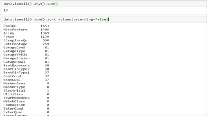
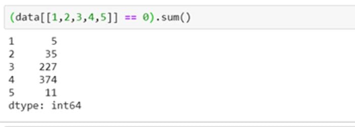
But, sometimes, it might not be this simple to identify missing values. One needs to use the domain knowledge and look at the data description to understand the variables. For instance, in the dataset below, isnull() does not show any null values.
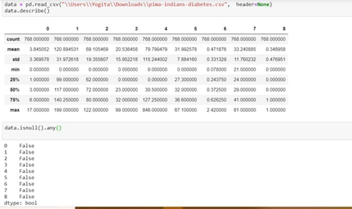
In this example, there are columns that have a minimum value of zero. On some columns, a value of zero does not make sense and indicates an invalid or missing value.
On analysing the features carefully, the following columns have an invalid zero minimum value:
- Plasma glucose concentration
- Diastolic blood pressure
- Triceps skinfold thickness
- 2-Hour serum insulin
- Body mass index
It becomes clear on checking the number of zeros in these columns that columns 1,2 and 5 have few zero values, whereas columns 3 and 4 have a lot more.
Missing values in each of these columns may need different strategies. We could mark these zero values as NaN to highlight missing values so that they could be processed further.
Quick classification of missing data
There are three types of missing data:
MCAR: Missing Completely At Random. It is the highest level of randomness. This means that the missing values in any features are not dependent on any other features values. This is the desirable scenario in case of missing data.
MAR: Missing At Random. This means that the missing values in any feature are dependent on the values of other features.
MNAR: Missing Not At Random. Missing not at random data is a more serious issue and in this case, it might be wise to check the data gathering process further and try to understand why the information is missing. For instance, if most of the people in a survey did not answer a certain question, why did they do that? Was the question unclear?
What to do with the missing values?
Now that we have identified the missing values in our data, next we should check the extent of the missing values to decide the further course of action.
Ignore the missing values
- Missing data under 10% for an individual case or observation can generally be ignored, except when the missing data is a MAR or MNAR.
- The number of complete cases i.e. observation with no missing data must be sufficient for the selected analysis technique if the incomplete cases are not considered.
Drop the missing values
Dropping a variable
- If the data is MCAR or MAR and the number of missing values in a feature is very high, then that feature should be left out of the analysis. If missing data for a certain feature or sample is more than 5% then you probably should leave that feature or sample out.
- If the cases or observations have missing values for target variables(s), it is advisable to delete the dependent variable(s) to avoid any artificial increase in relationships with independent variables.
Case Deletion
In this method, cases which have missing values for one or more features are deleted. If the cases having missing values are small in number, it is better to drop them. Though this is an easy approach, it might lead to a significant decrease in the sample size. Also, the data may not always be missing completely at random. This may lead to biased estimation of parameters.
Imputation
Imputation is the process of substituting the missing data by some statistical methods. Imputation is useful in the sense that it preserves all cases by replacing missing data with an estimated value based on other available information. But imputation methods should be used carefully as most of them introduce a large amount of bias and reduce variance in the dataset.
Imputation by Mean/Mode/Median
If the missing values in a column or feature are numerical, the values can be imputed by the mean of the complete cases of the variable. Mean can be replaced by median if the feature is suspected to have outliers. For a categorical feature, the missing values could be replaced by the mode of the column. The major drawback of this method is that it reduces the variance of the imputed variables. This method also reduces the correlation between the imputed variables and other variables because the imputed values are just estimates and will not be related to other values inherently.
Regression Methods
The variables with missing values are treated as dependent variables and variables with complete cases are taken as predictors or independent variables. The independent variables are used to fit a linear equation for the observed values of the dependent variable. This equation is then used to predict values for the missing data points.
The disadvantage of this method is that the identified independent variables would have a high correlation with the dependent variable by virtue of selection. This would result in fitting the missing values a little too well and reducing the uncertainty about that value. Also, this assumes that relationship is linear which might not be the case in reality.
K-Nearest Neighbour Imputation (KNN)
This method uses k-nearest neighbour algorithms to estimate and replace missing data. The k-neighbours are chosen using some distance measure and their average is used as an imputation estimate. This could be used for estimating both qualitative attributes (the most frequent value among the k nearest neighbours) and quantitative attributes (the mean of the k nearest neighbours).
One should try different values of k with different distance metrics to find the best match. The distance metric could be chosen based on the properties of the data. For example, Euclidean is a good distance measure to use if the input variables are similar in type (e.g. all measured widths and heights). Manhattan distance is a good measure to use if the input variables are not similar in type (such as age, gender, height, etc.).
The advantage of using KNN is that it is simple to implement. But it suffers from the curse of dimensionality. It works well for a small number of variables but becomes computationally inefficient when the number of variables is large.
Multiple Imputation
Multiple imputations is an iterative method in which multiple values are estimated for the missing data points using the distribution of the observed data. The advantage of this method is that it reflects the uncertainty around the true value and returns unbiased estimates.
MI involves the following three basic steps:
- Imputation: The missing data are filled in with estimated values and a complete data set is created. This process of imputation is repeated m times and m datasets are created.
- Analysis: Each of the m complete data sets is then analysed using a statistical method of interest (e.g. linear regression).
- Pooling: The parameter estimates (e.g. coefficients and standard errors) obtained from each analysed data set are then averaged to get a single point estimate.
Python’s Scikit-learn has methods — impute.SimpleImputer for univariate (single variable) imputations and impute.IterativeImputer for multivariate imputations.
The MICE package in R supports the multiple imputation functionality. Python does not directly support multiple imputations but IterativeImputer can be used for multiple imputations by applying it repeatedly to the same dataset with different random seeds when sample_posterior=True.
In summation, handling the missing data is crucial for a data science project. However, the data distribution should not be changed while handling missing data. Any missing data treatment method should satisfy the following rules:
- Estimation without bias — Any missing data treatment method should not change the data distribution.
- The relationship among the attributes should be retained.
Hope you enjoyed reading the blog!!
Please share your feedback and topics that you would like to know about.
References:
- https://machinelearningmastery.com/handle-missing-data-python/ https://en.wikipedia.org/wiki/Imputation_(statistics) https://stats.idre.ucla.edu/stata/seminars/mi_in_stata_pt1_new/
- https://pdfs.semanticscholar.org/e4f8/1aa5b67132ccf875cfb61946892024996413.pdf
Originally published at https://www.edvancer.in on July 2, 2019.
Bio: Yogita Kinha is a competent professional with experience in R, Python, Machine Learning and software environment for statistical computing and graphics, hands on experience on Hadoop ecosystem, and testing & reporting in software testing domain.
Original. Reposted with permission.
Related:
- Data Transformation: Standardization vs Normalization
- Simplified Mixed Feature Type Preprocessing in Scikit-Learn with Pipelines
- 5 Great New Features in Scikit-learn 0.23