How To Deal With Imbalanced Classification, Without Re-balancing the Data
Before considering oversampling your skewed data, try adjusting your classification decision threshold, in Python.
By David B Rosen (PhD), Lead Data Scientist for Automated Credit Approval at IBM Global Financing

Photo by Elena Mozhvilo on Unsplash
In machine learning, when building a classification model with data having far more instances of one class than another, the initial default classifier is often unsatisfactory because it classifies almost every case as the majority class. Many articles show you how you could use oversampling (e.g. SMOTE) or sometimes undersampling or simply class-based sample weighting to retrain the model on “rebalanced” data, but this isn’t always necessary. Here we aim instead to show how much you can do without balancing the data or retraining the model.
We do this by simply adjusting the the threshold for which we say “Class 1” when the model’s predicted probability of Class 1 is above it in two-class classification, rather than naïvely using the default classification rule which chooses which ever class is predicted to be most probable (probability threshold of 0.5). We will see how this gives you the flexibility to make any desired trade-off between false positive and false negative classifications while avoiding problems created by rebalancing the data.
We will use the credit card fraud identification data set from Kaggle to illustrate. Each row of the data set represents a credit card transaction, with the target variable Class==0 indicating a legitimate transaction and Class==1 indicating that the transaction turned out to be a fraud. There are 284,807 transactions, of which only 492 (0.173%) are frauds — very imbalanced indeed.
We will use a gradient boosting classifier because these often give good results. Specifically Scikit-Learn’s new HistGradientBoostingClassifier because it is much faster than their original GradientBoostingClassifier when the data set is relatively large like this one.
First let’s import some libraries and read in the data set.
import numpy as np
import pandas as pd
from sklearn import model_selection, metrics
from sklearn.experimental import enable_hist_gradient_boosting
from sklearn.ensemble import HistGradientBoostingClassifier
df=pd.read_csv('creditcard.csv')
df.info()
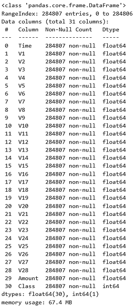
V1 through V28 (from a principal components analysis) and the transaction Amount are the features, which are all numeric and there is no missing data. Because we are only using a tree-based classifier, we don’t need to standardize or normalize the features.
We will now train the model after splitting the data into train and test sets. This took about half a minute on my laptop. We use the n_iter_no_change to stop the training early if the performance on a validation subset starts to deteriorate due to overfitting. I separately did a little bit of hyperparameter tuning to choose the learning_rate and max_leaf_nodes, but this is not the focus of the present article.
Xtrain, Xtest, ytrain, ytest = model_selection.train_test_split(
        df.loc[:,'V1':'Amount'], df.Class,  stratify=df.Class,
        test_size=0.3, random_state=42)
gbc=HistGradientBoostingClassifier(learning_rate=0.01,
        max_iter=2000, max_leaf_nodes=6, validation_fraction=0.2,
        n_iter_no_change=15, random_state=42).fit(Xtrain,ytrain)
Now we apply this model to the test data as the default hard-classifier, predicting 0 or 1 for each transaction. We are implicitly applying decision threshold 0.5 to the model’s continuous probability prediction as a soft-classifier. When the probability prediction is over 0.5 we say “1” and when it is under 0.5 we say “0”.
We also print the confusion matrix for the result, considering Class 1 (fraud) to be the “positive” class, by convention because it is the rarer class. The confusion matrix shows the number of True Negatives, False Positives, False Negatives, and True Positives. The normalized confusion matrix rates (e.g. FNR = False Negative Rate) are included as percentages in parentheses.
hardpredtst=gbc.predict(Xtest)
def conf_matrix(y,pred):
    ((tn, fp), (fn, tp)) = metrics.confusion_matrix(y, pred)
    ((tnr,fpr),(fnr,tpr))= metrics.confusion_matrix(y, pred,
            normalize='true')
    return pd.DataFrame([[f'TN = {tn} (TNR = {tnr:1.2%})',
                                f'FP = {fp} (FPR = {fpr:1.2%})'],
                         [f'FN = {fn} (FNR = {fnr:1.2%})',
                                f'TP = {tp} (TPR = {tpr:1.2%})']],
            index=['True 0(Legit)', 'True 1(Fraud)'],
            columns=['Pred 0(Approve as Legit)',
                            'Pred 1(Deny as Fraud)'])
conf_matrix(ytest,hardpredtst)
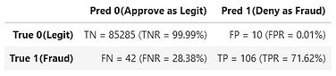
We see that the Recall for Class 1 (a.k.a. Sensitivity or True Positive Rate shown as TPR above) is only 71.62%, meaning that 71.62% of the true frauds are correctly identified as frauds and thus denied. So 28.38% of the true frauds are unfortunately approved as if legitimate.
Especially with imbalanced data (or generally any time false positives and false negatives may have different consequences), it’s important not to limit ourselves to using the default implicit classification decision threshold of 0.5, as we did above by using “.predict( )”. We want to improve the Recall of class 1 (the TPR) to reduce our fraud losses (reduce false negatives). To do this, we can reduce the threshold for which we say “Class 1” when we predict a probability above the threshold. This way we say “Class 1” for a wider range of predicted probabilities. Such strategies are known as threshold-moving.
Ultimately it is a business decision to what extent we want to reduce these False Negatives since as a trade-off the number of False Positives (true legitimate transactions rejected as frauds) will inevitably increase as we adjust the threshold that we apply to the model’s probability prediction (obtained from “.predict_proba( )” instead of “.predict( )”).
To elucidate this trade-off and help us choose a threshold, we plot the False Positive Rate and False Negative Rate against the Threshold. This is a variant of the Receiver Operating Characteristic (ROC) curve, but emphasizing the threshold.
predtst=gbc.predict_proba(Xtest)[:,1]
fpr, tpr, thresholds = metrics.roc_curve(ytest, predtst)
dfplot=pd.DataFrame({'Threshold':thresholds,
        'False Positive Rate':fpr,
        'False Negative Rate': 1.-tpr})
ax=dfplot.plot(x='Threshold', y=['False Positive Rate',
        'False Negative Rate'], figsize=(10,6))
ax.plot([0.00035,0.00035],[0,0.1]) #mark example thresh.
ax.set_xbound(0,0.0008); ax.set_ybound(0,0.3) #zoom in
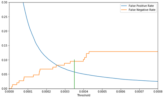
Although there exist some rules of thumb or proposed metrics for choosing the optimal threshold, ultimately it depends solely on the cost to the business of false negatives vs. false positives. For example, looking at the plot above, we might choose to apply a threshold of 0.00035 (vertical green line has been added) as follows.
hardpredtst_tuned_thresh = np.where(predtst >= 0.00035, 1, 0)
conf_matrix(ytest, hardpredtst_tuned_thresh)
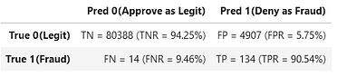
We have reduced our False Negative Rate from 28.38% down to 9.46% (i.e. identified and denied 90.54% of our true frauds as our new Recall or Sensitivity or True Positive Rate or TPR), while our False Positive Rate (FPR) has increased from 0.01% to 5.75% (i.e. still approved 94.25% of our legitimate transactions). It might well be worth the trade-off to us of denying about 6% of the legitimate transactions as the price we pay in order to approve only less than 10% of the fraudulent transactions, down from a very costly 28% of the frauds when we were using the default hard-classifier with an implicit classification decision threshold of 0.5.
Reasons not to balance your imbalanced data
One reason to avoid “balancing” your imbalanced training data is that such methods bias/distort the resulting trained model’s probability predictions so that these become miscalibrated, by systematically increasing the model’s predicted probabilities of the original minority class, and are thus reduced to being merely relative ordinal discriminant scores or decision functions or confidence scores rather than being potentially accurate predicted class probabilities in the original (“imbalanced”) train and test set and future data that the classifier may make predictions on. In the event that such rebalancing for training is truly needed, but numerically-accurate probability predictions are still desired, one would then have to recalibrate the predicted probabilities to a data set having the original/imbalanced class proportions. Alternatively you could apply a correction to the predicted probabilities from the balanced model — see Balancing is Unbalancing and this reply by its author.
Another problem with balancing your data by oversampling (as opposed to class-dependent instance weighting which doesn’t have this problem) is that it biases naïve cross-validation, potentially leading to excessive overfitting that is not detected in the cross-validation. In cross-validation, each time the data gets split into a “fold” subset, there may be instances in one fold that are duplicates of, or were generated from, instances in another fold. Thus the folds are not truly independent as cross-validation assumes — there is data “bleed” or “leakage”. For example see Cross-Validation for Imbalanced Datasets which describes how you could re-implement cross-validation correctly for this situation. However, in scikit-learn, at least for the case of oversampling by instance duplication (not necessarily SMOTE), this can alternatively be worked around by using model_selection.GroupKFold for cross-validation, which groups the instances according to a selected group identifier that has the same value for all duplicates of a given instance — see my reply to a response to the aforelinked article.
Conclusion
Instead of naïvely or implicitly applying a default threshold of 0.5, or immediately re-training using re-balanced training data, we can try using the original model (trained on the original “imbalanced” data set) and simply plot the trade-off between false positives and false negatives to choose a threshold that may produce a desirable business result.
Please leave a response if you have questions or comments.
Edit: Why does rebalancing your training data “work” even if the only real “problem” was that the default 0.5 threshold wasn’t appropriate?
The average probability prediction produced by your model will approximate the proportion of training instances that are class 1, because this is the average actual value of the target class variable (which has values of 0 and 1). The same is true in regression: the average predicted value of the target variable is expected to approximate the average actual value of the target variable. When the data is highly imbalanced and class 1 is the minority class, this average probability prediction will be much less than 0.5 and the vast majority of predictions of the probability of class 1 will be less than 0.5 and therefore classified as class 0 (majority class). If you rebalance the training data, the average predicted probability increases to 0.5 and so then many instances will be above a default threshold of 0.5 as well as many below — the predicted classes will be more balanced. So instead of reducing the threshold so that more often the probability predictions are above it and give class 1 (minority class), rebalancing increases the the predicted probabilities so that more often the probability predictions will be above the default threshold of 0.5 and give class 1.
If you want to get similar (not identical) results to those of rebalancing, without actually rebalancing or reweighting the data, you could try simply setting the threshold equal to the average or median value of the model’s predicted probability of class 1. But of course this won’t necessarily be the threshold that provides the optimal balance between false positives and false negatives for your particular business problem, nor will rebalancing your data and using a threshold of 0.5.
It is possible that there are situations and models where rebalancing the data will materially improve the model beyond merely moving the average predicted probability to equal the default threshold of 0.5. But the mere fact that the model chooses the majority class the vast majority of the time when using the default threshold of 0.5 does not in itself support a claim that rebalancing the data will accomplish anything beyond making the average probability prediction equal to the threshold. If you want the average probability prediction to be equal to the threshold, you could simply set the threshold equal to the average probability prediction, without modifying or reweighting your training data in order to distort the probability predictions.
Edit: Note about confidence scores vs. probability predictions
If your classifier doesn’t have a predict_proba method, e.g. support vector classifiers, you can just as well use its decision_function method in its place, producing an ordinal discriminant score or confidence score model output which can be thresholded in the same way even if it is not interpretable as a probability prediction between 0 and 1. Depending on how a particular classifier model calculates its confidence scores for the two classes, it might sometimes be necessary, instead of applying the threshold directly to the confidence score of class 1 (which we did above as the predicted probability of class 1 because the predicted probability of class 0 is simply one minus that), to alternatively apply the threshold to the difference between the confidence score for class 0 and that for class 1, with the default threshold being 0 for the case where the cost of a false positive is assumed to be the same as that of a false negative. This article assumes a two-class classification problem.
Bio: David B Rosen (PhD) is Lead Data Scientist for Automated Credit Approval at IBM Global Financing. Find more of David's writing at dabruro.medium.com.
Original. Reposted with permission.
Related:
- The 5 Most Useful Techniques to Handle Imbalanced Datasets
- Dealing with Imbalanced Data in Machine Learning
- Resampling Imbalanced Data and Its Limits