The 5 Most Useful Techniques to Handle Imbalanced Datasets
This post is about explaining the various techniques you can use to handle imbalanced datasets.
Have you ever faced an issue where you have such a small sample for the positive class in your dataset that the model is unable to learn?
In such cases, you get a pretty high accuracy just by predicting the majority class, but you fail to capture the minority class, which is most often the point of creating the model in the first place.
Such datasets are a pretty common occurrence and are called as an imbalanced dataset.
Imbalanced datasets are a special case for classification problem where the class distribution is not uniform among the classes. Typically, they are composed by two classes: The majority (negative) class and the minority (positive) class
Imbalanced datasets can be found for different use cases in various domains:
- Finance: Fraud detection datasets commonly have a fraud rate of ~1–2%
- Ad Serving: Click prediction datasets also don’t have a high clickthrough rate.
- Transportation/Airline: Will Airplane failure occur?
- Medical: Does a patient has cancer?
- Content moderation: Does a post contain NSFW content?
So how do we solve such problems?
This post is about explaining the various techniques you can use to handle imbalanced datasets.
1. Random Undersampling and Oversampling
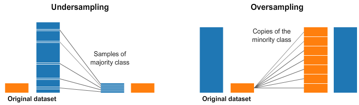
A widely adopted and perhaps the most straightforward method for dealing with highly imbalanced datasets is called resampling. It consists of removing samples from the majority class (under-sampling) and/or adding more examples from the minority class (over-sampling).
Let us first create some example imbalanced data.
from sklearn.datasets import make_classificationX, y = make_classification(
    n_classes=2, class_sep=1.5, weights=[0.9, 0.1],
    n_informative=3, n_redundant=1, flip_y=0,
    n_features=20, n_clusters_per_class=1,
    n_samples=100, random_state=10
)X = pd.DataFrame(X)
X['target'] = y
We can now do random oversampling and undersampling using:
num_0 = len(X[X['target']==0])
num_1 = len(X[X['target']==1])
print(num_0,num_1)# random undersampleundersampled_data = pd.concat([ X[X['target']==0].sample(num_1) , X[X['target']==1] ])
print(len(undersampled_data))# random oversampleoversampled_data = pd.concat([ X[X['target']==0] , X[X['target']==1].sample(num_0, replace=True) ])
print(len(oversampled_data))------------------------------------------------------------
OUTPUT:
90 10
20
180
2. Undersampling and Oversampling using imbalanced-learn
imbalanced-learn(imblearn) is a Python Package to tackle the curse of imbalanced datasets.
It provides a variety of methods to undersample and oversample.
a. Undersampling using Tomek Links:
One of such methods it provides is called Tomek Links. Tomek links are pairs of examples of opposite classes in close vicinity.
In this algorithm, we end up removing the majority element from the Tomek link, which provides a better decision boundary for a classifier.
from imblearn.under_sampling import TomekLinkstl = TomekLinks(return_indices=True, ratio='majority')X_tl, y_tl, id_tl = tl.fit_sample(X, y)
b. Oversampling using SMOTE:
In SMOTE (Synthetic Minority Oversampling Technique) we synthesize elements for the minority class, in the vicinity of already existing elements.

from imblearn.over_sampling import SMOTEsmote = SMOTE(ratio='minority')X_sm, y_sm = smote.fit_sample(X, y)
There are a variety of other methods in the imblearn package for both undersampling(Cluster Centroids, NearMiss, etc.) and oversampling(ADASYN and bSMOTE) that you can check out.
3. Class weights in the models

Most of the machine learning models provide a parameter called class_weights. For example, in a random forest classifier using, class_weights we can specify a higher weight for the minority class using a dictionary.
from sklearn.linear_model import LogisticRegressionclf = LogisticRegression(class_weight={0:1,1:10})
But what happens exactly in the background?
In logistic Regression, we calculate loss per example using binary cross-entropy:
Loss = −ylog(p) − (1−y)log(1−p)
In this particular form, we give equal weight to both the positive and the negative classes. When we set class_weight as class_weight = {0:1,1:20}, the classifier in the background tries to minimize:
NewLoss = −20*ylog(p) − 1*(1−y)log(1−p)
So what happens exactly here?
- If our model gives a probability of 0.3 and we misclassify a positive example, the NewLoss acquires a value of -20log(0.3) = 10.45
- If our model gives a probability of 0.7 and we misclassify a negative example, the NewLoss acquires a value of -log(0.3) = 0.52
That means we penalize our model around twenty times more when it misclassifies a positive minority example in this case.
How can we compute class_weights?
There is no one method to do this, and this should be constructed as a hyperparameter search problem for your particular problem.
But if you want to get class_weights using the distribution of the y variable, you can use the following nifty utility from sklearn.
from sklearn.utils.class_weight import compute_class_weightclass_weights = compute_class_weight('balanced', np.unique(y), y)
4. Change your Evaluation Metric

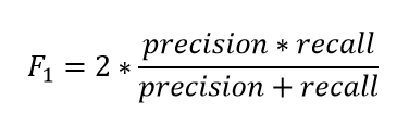
Choosing the right evaluation metric is pretty essential whenever we work with imbalanced datasets. Generally, in such cases, the F1 Score is what I want as my evaluation metric.
The F1 score is a number between 0 and 1 and is the harmonic mean of precision and recall.
So how does it help?
Let us start with a binary prediction problem. We are predicting if an asteroid will hit the earth or not.
So we create a model that predicts “No” for the whole training set.
What is the accuracy(Normally the most used evaluation metric)?
It is more than 99%, and so according to accuracy, this model is pretty good, but it is worthless.
Now, what is the F1 score?
Our precision here is 0. What is the recall of our positive class? It is zero. And hence the F1 score is also 0.
And thus we get to know that the classifier that has an accuracy of 99% is worthless for our case. And hence it solves our problem.
Simply stated the F1 score sort of maintains a balance between the precision and recall for your classifier. If your precision is low, the F1 is low, and if the recall is low again, your F1 score is low.
If you are a police inspector and you want to catch criminals, you want to be sure that the person you catch is a criminal (Precision) and you also want to capture as many criminals (Recall) as possible. The F1 score manages this tradeoff.
How to Use?
You can calculate the F1 score for binary prediction problems using:
from sklearn.metrics import f1_score
y_true = [0, 1, 1, 0, 1, 1]
y_pred = [0, 0, 1, 0, 0, 1]
f1_score(y_true, y_pred)
This is one of my functions which I use to get the best threshold for maximizing F1 score for binary predictions. The below function iterates through possible threshold values to find the one that gives the best F1 score.
# y_pred is an array of predictions
def bestThresshold(y_true,y_pred):
    best_thresh = None
    best_score = 0
    for thresh in np.arange(0.1, 0.501, 0.01):
        score = f1_score(y_true, np.array(y_pred)>thresh)
        if score > best_score:
            best_thresh = thresh
            best_score = score
    return best_score , best_thresh
5. Miscellaneous
Various other methods might work depending on your use case and the problem you are trying to solve:
a) Collect more Data
This is a definite thing you should try if you can. Getting more data with more positive examples is going to help your models get a more varied perspective of both the majority and minority classes.
b) Treat the problem as anomaly detection
You might want to treat your classification problem as an anomaly detection problem.
Anomaly detection is the identification of rare items, events or observations which raise suspicions by differing significantly from the majority of the data
You can use Isolation forests or autoencoders for anomaly detection.
c) Model-based
Some models are particularly suited for imbalanced datasets.
For example, in boosting models, we give more weights to the cases that get misclassified in each tree iteration.
Conclusion
There is no one size fits all when working with imbalanced datasets. You will have to try multiple things based on your problem.
In this post, I talked about the usual suspects that come to my mind whenever I face such a problem.
A suggestion would be to try using all of the above approaches and try to see whatever works best for your use case.
If you want to learn more about imbalanced datasets and the problems they pose, I would like to call out this excellent course by Andrew Ng. This was the one that got me started. Do check it out.
Thanks for the read. I am going to be writing more beginner-friendly posts in the future too. Follow me up at Medium or Subscribe to my blog to be informed about them. As always, I welcome feedback and constructive criticism and can be reached on Twitter @mlwhiz.
Also, a small disclaimer — There might be some affiliate links in this post to relevant resources, as sharing knowledge is never a bad idea.
Bio: Rahul Agarwal is Senior Statistical Analyst at WalmartLabs. Follow him on Twitter @mlwhiz.
Original. Reposted with permission.
Related:
- Classify A Rare Event Using 5 Machine Learning Algorithms
- The 5 Classification Evaluation Metrics Every Data Scientist Must Know
- The 5 Sampling Algorithms every Data Scientist need to know