Random Forest® — A Powerful Ensemble Learning Algorithm
The article explains the Random Forest algorithm and how to build and optimize a Random Forest classifier.
Introduction
In the article Decision Tree Algorithm — Explained, we have learned about Decision Tree and how it is used to predict the class or value of the target variable by learning simple decision rules inferred from prior data(training data).
But the common problem with Decision trees, especially having a table full of columns, they fit a lot. Sometimes it looks like the tree memorized the training data set. If there is no limit set on a decision tree, it will give you 100% accuracy on the training data set because in the worse case it will end up making 1 leaf for each observation. Thus this affects the accuracy when predicting samples that are not part of the training set.
Random forest is one of several ways to solve this problem of overfitting, now let us dive deeper into the working and implementation of this powerful machine learning algorithm. But before that, I would suggest you get familiar with the Decision tree algorithm.
Random forest is an ensemble learning algorith, so before talking about random forest let us first briefly understand what are Ensemble Learning algorithms.
Ensemble Learning algorithms
Ensemble learning algorithms are meta-algorithms that combine several machine learning algorithms into one predictive model in order to decrease variance, bias or improve predictions.
The algorithm can be any machine learning algorithm such as logistic regression, decision tree, etc. These models, when used as inputs of ensemble methods, are called ”base models”.
Ensemble methods usually produce more accurate solutions than a single model would. This has been the case in a number of machine learning competitions, where the winning solutions used ensemble methods. In the popular Netflix Competition, the winner used an ensemble method to implement a powerful collaborative filtering algorithm. Another example is KDD 2009 where the winner also used ensemble methods.
Ensemble algorithms or methods can be divided into two groups:
- Sequential ensemble methods — where the base learners are generated sequentially (e.g. AdaBoost).
The basic motivation of sequential methods is to exploit the dependence between the base learners. The overall performance can be boosted by weighing previously mislabeled examples with higher weight. - Parallel ensemble methods — where the base learners are generated in parallel (e.g. Random Forest).
The basic motivation of parallel methods is to exploit independence between the base learners since the error can be reduced dramatically by averaging.
Most ensemble methods use a single base learning algorithm to produce homogeneous base learners, i.e. learners of the same type, leading to homogeneous ensembles.
There are also some methods that use heterogeneous learners, i.e. learners of different types, leading to heterogeneous ensembles. In order for ensemble methods to be more accurate than any of its individual members, the base learners have to be as accurate as possible and as diverse as possible.
What is the Random Forest algorithm?
Random forest is a supervised ensemble learning algorithm that is used for both classifications as well as regression problems. But however, it is mainly used for classification problems. As we know that a forest is made up of trees and more trees mean more robust forest. Similarly, the random forest algorithm creates decision trees on data samples and then gets the prediction from each of them and finally selects the best solution by means of voting. It is an ensemble method that is better than a single decision tree because it reduces the over-fitting by averaging the result.

The fundamental concept behind random forest is a simple but powerful one — the wisdom of crowds.
“A large number of relatively uncorrelated models(trees) operating as a committee will outperform any of the individual constituent models.”
The low correlation between models is the key.
The reason why Random forest produces exceptional results is that the trees protect each other from their individual errors. While some trees may be wrong, many others will be right, so as a group the trees are able to move in the correct direction.
Why the name “Random”?
Two key concepts that give it the name random:
- A random sampling of training data set when building trees.
- Random subsets of features considered when splitting nodes.
How is Random Forest ensuring Model diversity?
Random forest ensures that the behavior of each individual tree is not too correlated with the behavior of any other tree in the model by using the following two methods:
- Bagging or Bootstrap Aggregation
- Random feature selection
Bagging or Bootstrap Aggregation
Decision trees are very sensitive to the data they are trained on, small changes to the training data set can result in a significantly different tree structure. The random forest takes advantage of this by allowing each individual tree to randomly sample from the dataset with replacement, resulting in different trees. This process is called Bagging.
Note that with bagging we are not subsetting the training data into smaller chunks and training each tree on a different chunk. Rather, if we have a sample of size N, we are still feeding each tree a training set of size N. But instead of the original training data, we take a random sample of size N with replacement.
For example — If our training data is [1,2,3,4,5,6], then we might give one of our trees the list [1,2,2,3,6,6] and we can give another tree a list [2,3,4,4,5,6]. Notice that the lists are of length 6 and some elements are repeated in the randomly selected training data we can give to our tree(because we sample with replacement).
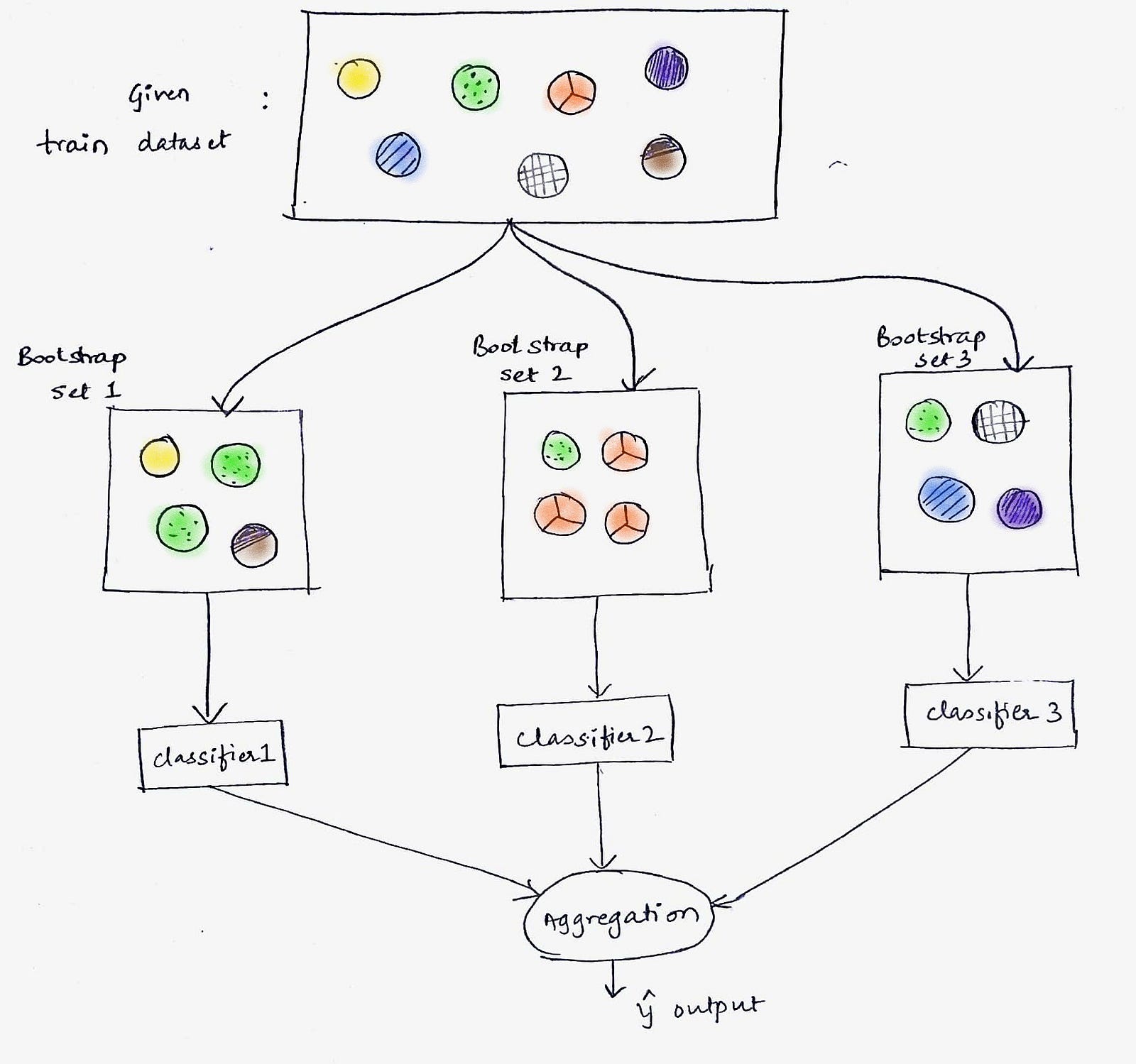
The above figure shows how random samples are taken from the dataset with replacement.
Random feature selection
In a normal decision tree, when it is time to split a node, we consider every possible feature and pick the one that produces the most separation between the observations in the left node vs right node. In contrast, each tree in a random forest can pick only from a random subset of features. This forces even more variation amongst the trees in the model and ultimately results in low correlation across trees and more diversification.
So in random forest, we end up with trees that are trained on different sets of data and also use different features to make decisions.
And finally, uncorrelated trees have created that buffer and predict each other from their respective errors.
Random Forest creation pseudocode:
- Randomly select “k” features from total “m” features where k << m
- Among the “k” features, calculate the node “d” using the best split point
- Split the node into daughter nodes using the best split
- Repeat the 1 to 3 steps until “l” number of nodes has been reached
- Build forest by repeating steps 1 to 4 for “n” number times to create “n” number of trees.
Random Forest classifier Building in Scikit-learn
In this section, we are going to build a Gender Recognition classifier using the Random Forest algorithm from the voice dataset. The idea is to identify a voice as male or female, based upon the acoustic properties of the voice and speech. The dataset consists of 3,168 recorded voice samples, collected from male and female speakers. The voice samples are pre-processed by acoustic analysis in R using the seewave and tuneR packages, with an analyzed frequency range of 0hz-280hz.
The dataset can be downloaded from kaggle.
The goal is to create a Decision tree and Random Forest classifier and compare the accuracy of both the models. The following are the steps that we will perform in the process of model building:
1. Importing Various Modules and Loading the Dataset
2. Exploratory Data Analysis (EDA)
3. Outlier Treatment
4. Feature Engineering
5. Preparing the Data
6. Model building
7. Model optimization
So let us start.
Step-1: Importing Various Modules and Loading the Dataset
# Ignore  the warnings
import warnings
warnings.filterwarnings('always')
warnings.filterwarnings('ignore')# data visualisation and manipulationimport numpy as np
import pandas as pd
import matplotlib.pyplot as plt
from matplotlib import style
import seaborn as sns
import missingno as msno#configure
# sets matplotlib to inline and displays graphs below the corressponding cell.
%matplotlib inline
style.use('fivethirtyeight')
sns.set(style='whitegrid',color_codes=True)#import the necessary modelling algos.
from sklearn.ensemble import RandomForestClassifier
from sklearn.tree import DecisionTreeClassifier

#model selection
from sklearn.model_selection import train_test_split
from sklearn.model_selection import KFold
from sklearn.metrics import accuracy_score,precision_score
from sklearn.model_selection import GridSearchCV#preprocess.
from sklearn.preprocessing import MinMaxScaler,StandardScaler
Now load the dataset.
train=pd.read_csv("../RandomForest/voice.csv")df=train.copy()
Step-2: Exploratory Data Analysis (EDA)
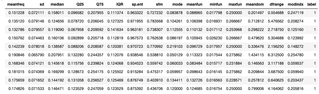
df.head(10)
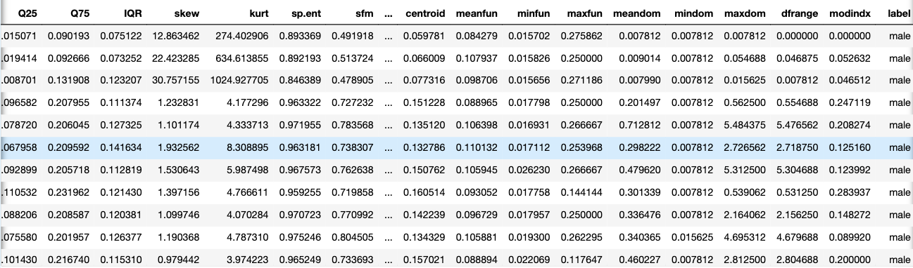
The following acoustic properties of each voice are measured and included within our data:
- meanfreq: mean frequency (in kHz)
- sd: standard deviation of the frequency
- median: median frequency (in kHz)
- Q25: first quantile (in kHz)
- Q75: third quantile (in kHz)
- IQR: interquartile range (in kHz)
- skew: skewness
- kurt: kurtosis
- sp.ent: spectral entropy
- sfm: spectral flatness
- mode: mode frequency
- centroid: frequency centroid
- peakf: peak frequency (the frequency with the highest energy)
- meanfun: the average of fundamental frequency measured across an acoustic signal
- minfun: minimum fundamental frequency measured across an acoustic signal
- maxfun: maximum fundamental frequency measured across an acoustic signal
- meandom: the average of dominant frequency measured across an acoustic signal
- mindom: minimum of dominant frequency measured across an acoustic signal
- maxdom: maximum of dominant frequency measured across an acoustic signal
- dfrange: the range of dominant frequency measured across an acoustic signal
- modindx: modulation index which is calculated as the accumulated absolute difference between adjacent measurements of fundamental frequencies divided by the frequency range
- label: male or female
df.shape
Note that we have 3168 voice samples and for each sample, 20 different acoustic properties are recorded. Finally, the ‘label’ column is the target variable which we have to predict which is the gender of the person.
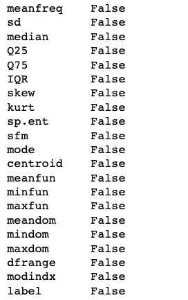
Now our next step is handling the missing values.
# check for null values.
df.isnull().any()
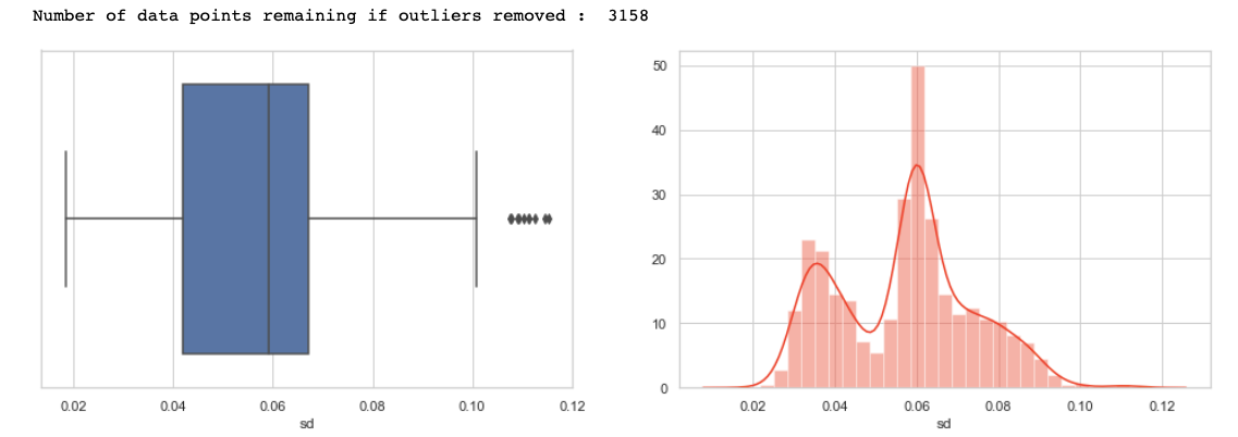
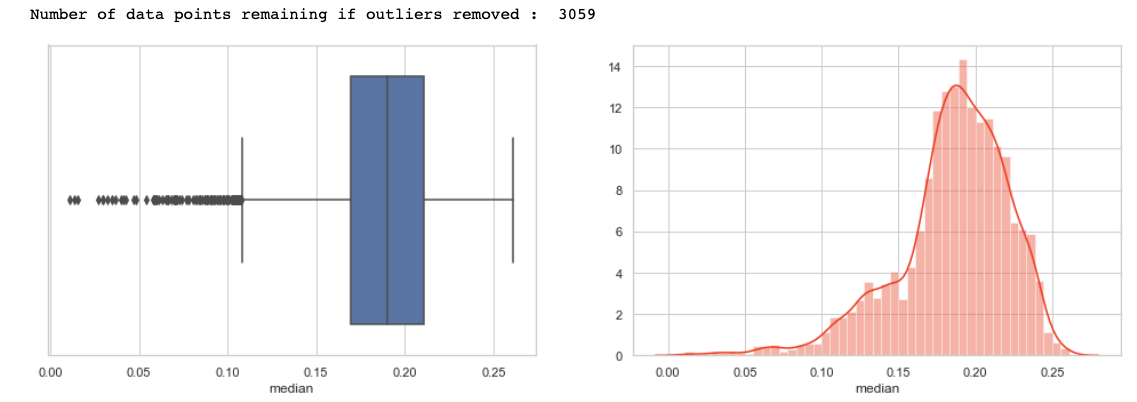
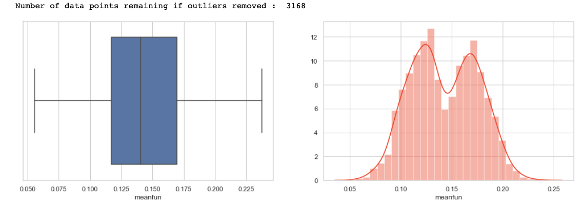
Now I will perform the univariate analysis. Note that since all of the features are ‘numeric’ the most reasonable way to plot them would either be a ‘histogram’ or a ‘boxplot’.
Also, univariate analysis is useful for outlier detection. Hence besides plotting a boxplot and a histogram for each column or feature, I have written a small utility function that tells the remaining no. of observations for each feature if we remove its outliers.
To detect the outliers I have used the standard 1.5 InterQuartileRange (IQR) rule which states that any observation lesser than ‘first quartile — 1.5 IQR’ or greater than ‘third quartile +1.5 IQR’ is an outlier.
def calc_limits(feature):
    q1,q3=df[feature].quantile([0.25,0.75])
    iqr=q3-q1
    rang=1.5*iqr
    return(q1-rang,q3+rang)

def plot(feature):
    fig,axes=plt.subplots(1,2)
    sns.boxplot(data=df,x=feature,ax=axes[0])
    sns.distplot(a=df[feature],ax=axes[1],color='#ff4125')
    fig.set_size_inches(15,5)

    lower,upper = calc_limits(feature)
    l=[df[feature] for i in df[feature] if i>lower and i<upper]
    print("Number of data points remaining if outliers removed : ",len(l))
Let us plot the first feature i.e. meanfreq.
plot('meanfreq')
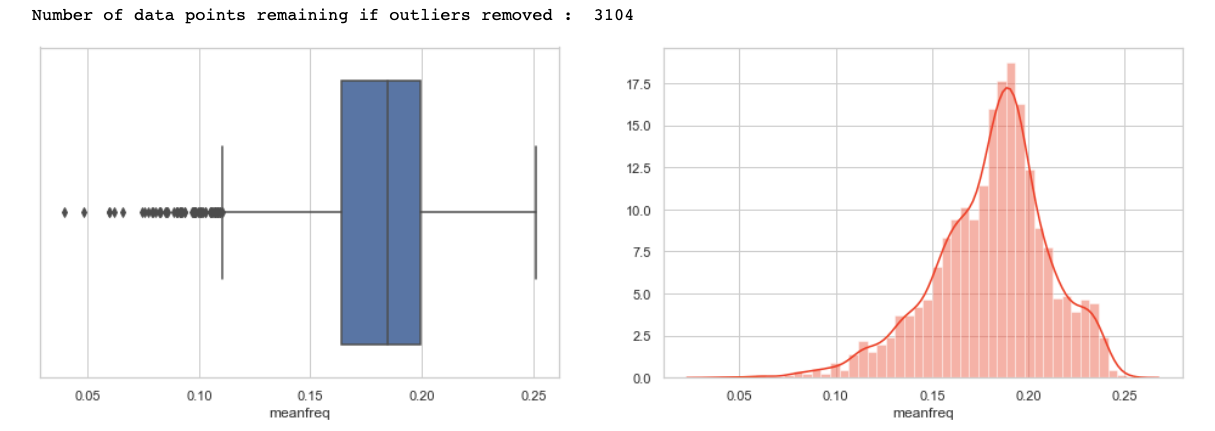
Inferences made from the above plots —
1) First of all, note that the values are in compliance with that observed from describing the method data frame.
2) Note that we have a couple of outliers w.r.t. to 1.5 quartile rule (represented by a ‘dot’ in the box plot). Removing these data points or outliers leaves us with around 3104 values.
3) Also, from the distplot that the distribution seems to be a bit -ve skewed hence we can normalize to make the distribution a bit more symmetric.
4) LASTLY, NOTE THAT A LEFT TAIL DISTRIBUTION HAS MORE OUTLIERS ON THE SIDE BELOW TO Q1 AS EXPECTED AND A RIGHT TAIL HAS ABOVE THE Q3.
Similar inferences can be made by plotting other features also, I have plotted some, you guys can check for all.
Now plot and count the target variable to check if the target class is balanced or not.
sns.countplot(data=df,x='label')
df['label'].value_counts()
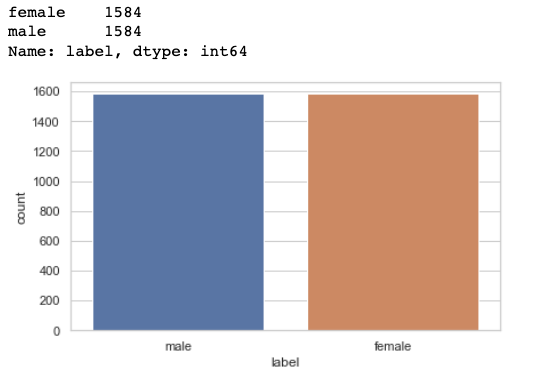
We have the equal number of observations for the ‘males’ and the ‘females’ class hence it is a balanced dataset and we don't need to do anything about it.
Now I will perform Bivariate analysis to analyze the correlation between different features. To do it I have plotted a ‘heat map’ which clearly visualizes the correlation between different features.
temp = []
for i in df.label:
    if i == 'male':
        temp.append(1)
    else:
        temp.append(0)
df['label'] = temp
#corelation matrix.
cor_mat= df[:].corr()
mask = np.array(cor_mat)
mask[np.tril_indices_from(mask)] = False
fig=plt.gcf()
fig.set_size_inches(23,9)
sns.heatmap(data=cor_mat,mask=mask,square=True,annot=True,cbar=True)
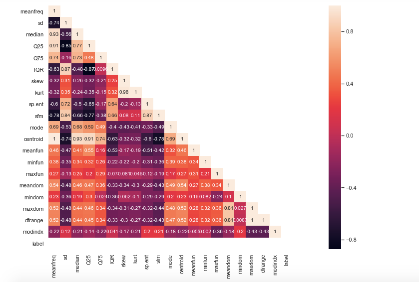
Inferences made from above heatmap plot—
1) Mean frequency is moderately related to label.
2) IQR and label tend to have a strong positive correlation.
3) Spectral entropy is also quite highly correlated with the label while sfm is moderately related with label.
4) skewness and kurtosis aren’t much related to label.
5) meanfun is highly negatively correlated with the label.
6) Centroid and median have a high positive correlation expected from their formulae.
7) Also, meanfreq and centroid are exactly the same features as per formulae and so are the values. Hence their correlation is perfect 1. In this case, we can drop any of that column.
Note that centroid in general has a high degree of correlation with most of the other features so I’m going to drop centroid column.
8) sd is highly positively related to sfm and so is sp.ent to sd.
9) kurt and skew are also highly correlated.
10) meanfreq is highly related to the median as well as Q25.
11) IQR is highly correlated to sd.
12) Finally, self relation ie of a feature to itself is equal to 1 as expected.
Note that we can drop some highly correlated features as they add redundancy to the model but let us keep all the features for now. In the case of highly correlated features, we can use dimensionality reduction techniques like Principal Component Analysis(PCA) to reduce our feature space.
df.drop('centroid',axis=1,inplace=True)
Step-3: Outlier Treatment
Here we have to deal with the outliers. Note that we discovered the potential outliers in the ‘univariate analysis’ section. Now to remove those outliers we can either remove the corresponding data points or impute them with some other statistical quantity like median (robust to outliers) etc.
For now, I shall be removing all the observations or data points that are an outlier to ‘any’ feature. Doing so substantially reduces the dataset size.
# removal of any data point which is an outlier for any fetaure.
for col in df.columns:
    lower,upper=calc_limits(col)
    df = df[(df[col] >lower) & (df[col]<upper)]df.shape
Note that the new shape is (1636, 20), we are left with 20 features.
Step-4: Feature Engineering
Here I have dropped some columns which according to my analysis proved to be less useful or redundant.
temp_df=df.copy()temp_df.drop(['skew','kurt','mindom','maxdom'],axis=1,inplace=True) # only one of maxdom and dfrange.
temp_df.head(10)
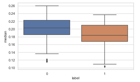
Now let us create some new features. I have done two new things here. Firstly I have made ‘meanfreq’, ’median’ and ‘mode’ to comply with the standard relation 3Median=2Mean +Mode. For this, I have adjusted values in the ‘median’ column as shown below. You can alter values in any of the other columns say the ‘meanfreq’ column.
temp_df['meanfreq']=temp_df['meanfreq'].apply(lambda x:x*2)
temp_df['median']=temp_df['meanfreq']+temp_df['mode']
temp_df['median']=temp_df['median'].apply(lambda x:x/3)sns.boxplot(data=temp_df,y='median',x='label') # seeing the new 'median' against the 'label'
The second new feature that I have added is a new feature to measure the ‘skewness’.
For this, I have used the ‘Karl Pearson Coefficient’ which is calculated as Coefficient = (Mean — Mode )/StandardDeviation
You can also try some other coefficient also and see how it compared with the target i.e. the ‘label’ column.
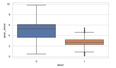
temp_df['pear_skew']=temp_df['meanfreq']-temp_df['mode']
temp_df['pear_skew']=temp_df['pear_skew']/temp_df['sd']
temp_df.head(10)sns.boxplot(data=temp_df,y='pear_skew',x='label')
Step-5: Preparing the Data
The first thing that we’ll do is normalize all the features or basically we’ll perform feature scaling to get all the values in a comparable range.
scaler=StandardScaler()
scaled_df=scaler.fit_transform(temp_df.drop('label',axis=1))
X=scaled_df
Y=df['label'].as_matrix()
Next split your data into train and test set.
x_train,x_test,y_train,y_test=train_test_split(X,Y,test_size=0.20,random_state=42)
Step-6: Model building
Now we’ll build two classifiers, decision tree, and random forest and compare the accuracies of both of them.
models=[RandomForestClassifier(), DecisionTreeClassifier()]model_names=['RandomForestClassifier','DecisionTree']acc=[]
d={}for model in range(len(models)):
    clf=models[model]
    clf.fit(x_train,y_train)
    pred=clf.predict(x_test)
    acc.append(accuracy_score(pred,y_test))

d={'Modelling Algo':model_names,'Accuracy':acc}
Put the accuracies in a data frame.
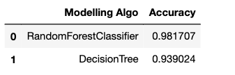
acc_frame=pd.DataFrame(d)
acc_frame
Plot the accuracies:
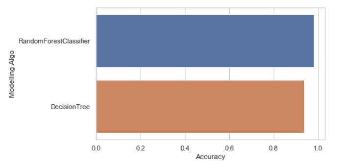
As we have seen, just by using the default parameters for both of our models, the random forest classifier outperformed the decision tree classifier(as expected).
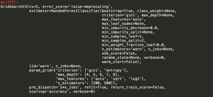
Step-7: Parameter Tuning with GridSearchCV
Lastly, let us also tune our random forest classifier using GridSearchCV.
param_grid = {
    'n_estimators': [200, 500],
    'max_features': ['auto', 'sqrt', 'log2'],
    'max_depth' : [4,5,6,7,8],
    'criterion' :['gini', 'entropy']
}
CV_rfc = GridSearchCV(estimator=RandomForestClassifier(), param_grid=param_grid, scoring='accuracy', cv= 5)
CV_rfc.fit(x_train, y_train)
print("Best score : ",CV_rfc.best_score_)
print("Best Parameters : ",CV_rfc.best_params_)
print("Precision Score : ", precision_score(CV_rfc.predict(x_test),y_test))

After hyperparameter optimization as we can see the results are pretty good :)
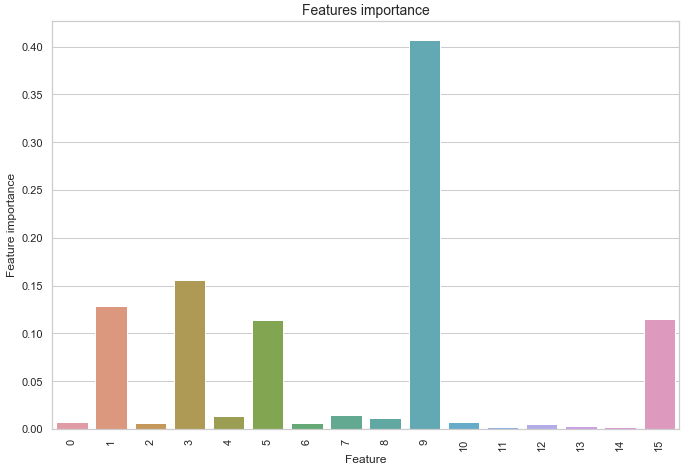
If you want you can also check the Importance of each feature.
df1 = pd.DataFrame.from_records(x_train)
tmp = pd.DataFrame({'Feature': df1.columns, 'Feature importance': clf_rf.feature_importances_})
tmp = tmp.sort_values(by='Feature importance',ascending=False)
plt.figure(figsize = (7,4))
plt.title('Features importance',fontsize=14)
s = sns.barplot(x='Feature',y='Feature importance',data=tmp)
s.set_xticklabels(s.get_xticklabels(),rotation=90)
plt.show()
Conclusion
Now that you hopefully have the conceptual framework of random forest and this article has given you the confidence and understanding needed to start using the random forest on your projects. The random forest is a powerful machine learning model, but that should not prevent us from knowing how it works. The more we know about a model, the better equipped we will be to use it effectively and explain how it makes predictions.
You can find the source code in my Github repository.
Well, that’s all for this article hope you guys have enjoyed reading it and I’ll be glad if the article is of any help. Feel free to share your comments/thoughts/feedback in the comment section.
Thanks for reading!!!
Bio: Nagesh Singh Chauhan is a Big data developer at CirrusLabs. He has over 4 years of working experience in various sectors like Telecom, Analytics, Sales, Data Science having specialisation in various Big data components.
Original. Reposted with permission.
Random Forests® is a registered trademark of Minitab.
Related:
- A Friendly Introduction to Support Vector Machines
- Comparing Decision Tree Algorithms: Random Forest vs. XGBoost
- Build an Artificial Neural Network From Scratch: Part 1