Easy Guide To Data Preprocessing In Python
Preprocessing data for machine learning models is a core general skill for any Data Scientist or Machine Learning Engineer. Follow this guide using Pandas and Scikit-learn to improve your techniques and make sure your data leads to the best possible outcome.

Image by rawpixel.com on Freepik
Machine Learning is 80% preprocessing and 20% model making.
You must have heard this phrase if you have ever encountered a senior Kaggle data scientist or machine learning engineer. The fact is that this is a true phrase. In a real-world data science project, data preprocessing is one of the most important things, and it is one of the common factors of success of a model, i.e., if there is correct data preprocessing and feature engineering, that model is more likely to produce noticeably better results as compared to a model for which data is not well preprocessed.
Important Steps
There are 4 main important steps for the preprocessing of data.
- Splitting of the data set in Training and Validation sets
- Taking care of Missing values
- Taking care of Categorical Features
- Normalization of data set
Let’s have a look at all of these points.
1. Train Test Split
Train Test Split is one of the important steps in Machine Learning. It is very important because your model needs to be evaluated before it has been deployed. And that evaluation needs to be done on unseen data because when it is deployed, all incoming data is unseen.
The main idea behind the train test split is to convert original data set into 2 parts
- train
- test
where train consists of training data and training labels and test consists of testing data and testing labels.
The easiest way to do it is by using scikit-learn, which has a built-in function train_test_split. Let’s code it.
from sklearn.model_selection import train_test_split

X_train, X_test, y_train, y_test = train_test_split(X, y, test_size = 0.2)
Here we have passed-in X and y as arguments in train_test_split, which splits X and y such that there is 20% testing data and 80% training data successfully split between X_train, X_test, y_train, and y_test.
2. Taking Care of Missing Values
There is a famous Machine Learning phrase which you might have heard that is
Garbage in Garbage out
If your data set is full of NaNs and garbage values, then surely your model will perform garbage too. So taking care of such missing values is important. Let’s take a dummy data set to see how we can tackle this problem of taking care of garbage values. You can get that data set here.
Let’s see the missing values in the data set.
df.isna().sum()
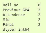
Here we can see that we have 2 missing values in 4 columns. One approach to fill in missing values is to fill it with the mean of that column, which is the average of that column. For example, we can fill in the missing value of Final column by an average of all students in that column.
To do that, we can use SimpleImputer from sklearn.impute.
from sklearn.impute import SimpleImputer

imputer = SimpleImputer(fill_value=np.nan, startegy='mean')
X = imputer.fit_transform(df)
This will fill all the missing values in the data frame df using mean of that column. We use the fit_transform function to do that.
Because it returns a numpy array, to read it, we can convert it back to the data frame.
X = pd.DataFrame(X, columns=df.columns)
print(X)
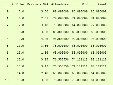
And now, we can see that we have filled all the missing values by mean of all values.
We can confirm it by
X.isna().sum()
and the output is
We can use mean, meadian, mode etc. in SimpleImputer.
If our number of rows which have missing values are less, or our data is such that it is not advised to fill in missing values, then we can drop the missing rows by using dropna in pandas.
dropedDf = df.dropna()
And here, we have dropped all the null rows in the dataframe and stored it in another dataframe.
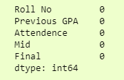
Now we have 0 null rows as we have dropped them. We can confirm it as
dropedD.isna().sum()
3. Taking care of Categorical Features
We can take care of categorical features by converting them to integers. There are 2 common ways to do so.
- Label Encoding
- One Hot Encoding
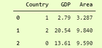
In Label Encoder, we can convert the Categorical values into numerical labels. Let’s say this is our dataset
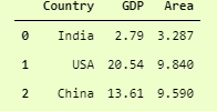
and using label encoder on the Country column will convert India to 1, the USA to 2, and China to 0. This technique has a drawback that it gives the USA the highest priority due to its label is high and China the lowest priority for its label being 0, but still, it is helping a lot of times.
Let’s code it.
from sklearn.preprocessing import LabelEncoder

l1 = LabelEncoder()
l1.fit(catDf['Country'])
catDf.Country = l1.transform(catDf.Country)
print(catDf)
Output after Label Encoder
Here we have instantiated a LabelEncoder object, then used the fit method to fit it on our categorical column and then used transform method to apply it.
Note that it is not inplace so in order to make the change permanent, we have to return the value to our categorical column, i.e.,
catDf['Country'] = l1.transform(catDf['Country'])
In OneHotEncoder we make a new column for each unique categorical value, and the value is 1 for that column, if in an actual data frame that value is there, else it is 0.
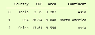
Let’s See it with the same example but a bit modified. We will add another categorical column, which is “Continent,” that has the name of the continent of the respective country. We can do it by
catDf['Continent'] = ['Asia', 'North America', 'Asia']
Now because we have 2 categorical columns, which are [['Country', 'Continent']], we can one hot encode them.
There are 2 ways to do so.
1. DataFrame.get_dummies
This is a pretty common way where we use pandas built-in function get_dummies to convert categorical values in a dataframe to a one-hot vector.
Let’s do this.
pd.get_dummies(data=catDf)
This will return a data frame with all the categorical values encoded in a one-hot vector format.
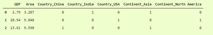
Here we can see that it has converted the unique values of Country columns as 3 different columns, which are Country_China, Country_India, and Country_USA. Similarly, 2 unique values of Continent Column has been converted into 2 different columns named as Continent_Asia and Continent_North America.
Because it is not in place, we have to either store it in a data frame, i.e.,
catDf = pd.get_dummies(data=catDf)
2. OneHotEncoder
Using OneHotEncoder from Sci-Kit Learning is also a common practice. It does provide more flexibility and more options but is a bit difficult to use. Let’s see how we can do it for our dataset.
from sklearn.preprocessing import OneHotEncoder

oh = OneHotEncoder()
s1 = pd.DataFrame(oh.fit_transform(catDf.iloc[:, [0,3]]))
pd.concat([catDf, s1], axis=1)
Here, we have initialized OneHotEncoder Object and used its fit_transform method on our desired columns (column number 0 and column number 3) in the data frame.
The return type of fit_transform is numpy.ndarray, so we convert it into a dataframe by pd.DataFrame and stored it in a variable. Then, to join it in our original data frame, we can use pd.concat the function that concatenates 2 different data frames. We have used axis=1, which means it has to join on the basis of columns instead of rows.
Also, remember that pd.concat is not inplace, so we have to store the returning dataframe somewhere.
catDf = pd.concat([catDf, s1], axis=1)
The resulting dataframe is
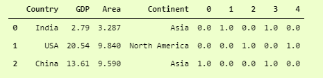
OneHotEncoded DataFrame
You can see that it is not clearly readable as compared to pd.get_dummies, but if you compare the last 5 columns that we got using pd.get_dummies and OneHotEncoder, then they are all equal.
Of course, you can modify the column names as per your choice in OneHotEncoder, which you can learn as per this question from StackOverflow.
4. Normalizing the Dataset
This brings us to the last part of data preprocessing, which is the normalization of the dataset. It is proven from certain experimentation that Machine Learning and Deep Learning Models perform way better on a normalized data set as compared to a data set that is not normalized.
The goal of normalization is to change values to a common scale without distorting the difference between the range of values.
There are several ways to do so. I will discuss 2 common ways to normalize a dataset.
Standard Scaler
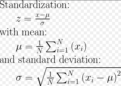
Credit: https://stackoverflow.com/a/50879522/10342778
Using this technique, we are going to have a mean of 0 and a standard deviation of 1 in our dataset. We can either do it normally by combining different functions in numpy, i.e.,
z = (x.values - np.mean(x.values)) / np.std(x.values)
where x is a dataframe with all numerical indices. If we want to retain the values in a dataframe, then we can simply remove .values in front of it.
Variance before StandardScaler
catDf.var(ddof=0)
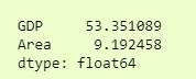
var before StandardScaler.
Here, I have used ddof=0, which is by default 1 in pandas.DataFrame.var() and by default 0 in numpy.ndarray.var(). Ddof means Delta Degrees of Freedom, which is the divisor used in calculations is N - ddof, where N represents the number of elements.
ddof=0 provides a maximum likelihood estimate of the variance for normally distributed variables.
You can read more about ddof=0 here.
Variance after StandardScaler
Another good way to do so by using StandardScaler from sklearn.preprocessing. Let’s see the code, and then see the variance.
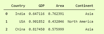
from sklearn.preprocessing import StandardScaler

ss = StandardScaler()
catDf.iloc[:,1:-1] = ss.fit_transform(catDf.iloc[:,1:-1])
print(catDf)
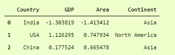
catDf after StandardScaler.
Here we have applied StandardScaler on all the numerical columns (column number 1 to the last column (not included)), and now you can see the values of GDP and Area.
Now we can check the variance of the dataset by
catDf.var(ddof=0)
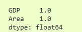
var after StandardScaler
And we can see the massive reduction of the variance of 80 and 13 to 1. In real-world datasets, normally the improvement is from thousands to 1.
Normalization
According to the official documentation of sklearn, normalization is “the process of scaling individual samples to have unit norm. This process can be useful if you plan to use a quadratic form such as the dot-product or any other kernel to quantify the similarity of any pair of samples.”
The process of using it is very simple and similar to StandaradScaler.
from sklearn.preprocessing import Normalizer

norm = Normalizer()
catDf.iloc[:,1:-1] = norm.fit_transform(catDf.iloc[:,1:-1])
catDf
catDf after Normalizer
There are several other ways to normalize the data, and all of them are useful in specific cases. You can read more about them in the official documentation here.
Learning Outcomes
- Splitting the Dataset
- Filling in Missing values
- Dealing with Categorical Data
- Normalization of Dataset for improved results
Hopefully, all these techniques will improve your general skills as a data scientist or machine learning engineer and will improve your Machine Learning Models.
Ahmad Anis is interested in Machine Learning, Deep Learning, and Computer Vision. Currently working as a Jr. Machine Learning engineer at Redbuffer.