7 Steps to Mastering Data Cleaning and Preprocessing Techniques
Are you trying to solve your first data science project? This tutorial will help you to guide you step by step to prepare your dataset before applying the machine learning model.
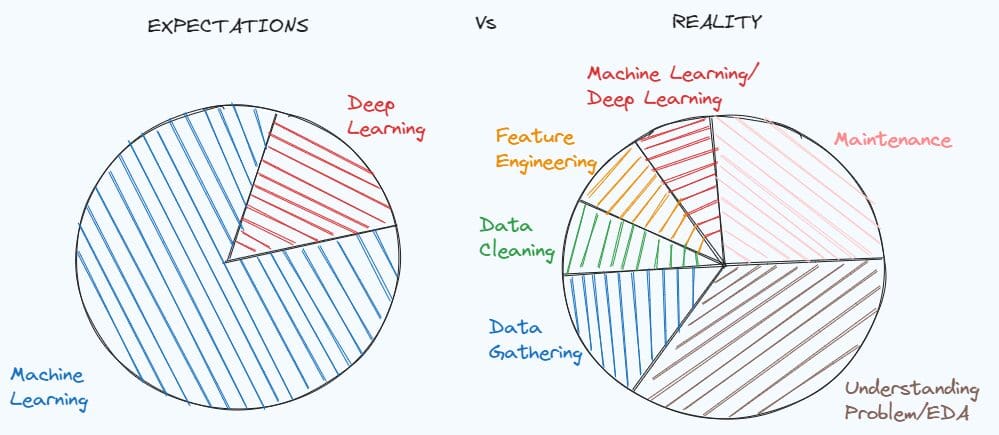
Illustration by Author. Inspired by MEME of Dr. Angshuman Ghosh
Mastering Data Cleaning and Preprocessing Techniques is fundamental for solving a lot of data science projects. A simple demonstration of how important can be found in the meme about the expectations of a student studying data science before working, compared with the reality of the data scientist job.
We tend to idealise the job position before having a concrete experience, but the reality is that it’s always different from what we really expect. When working with a real-world problem, there is no documentation of the data and the dataset is very dirty. First, you have to dig deep in the problem, understand what clues you are missing and what information you can extract.
After understanding the problem, you need to prepare the dataset for your machine learning model since the data in its initial condition is never enough. In this article, I am going to show seven steps that can help you on pre-processing and cleaning your dataset.
Step 1: Exploratory Data Analysis
The first step in a data science project is the exploratory analysis, that helps in understanding the problem and taking decisions in the next steps. It tends to be skipped, but it’s the worst error because you’ll lose a lot of time later to find the reason why the model gives errors or didn’t perform as expected.
Based on my experience as data scientist, I would divide the exploratory analysis into three parts:
- Check the structure of the dataset, the statistics, the missing values, the duplicates, the unique values of the categorical variables
- Understand the meaning and the distribution of the variables
- Study the relationships between variables
To analyse how the dataset is organised, there are the following Pandas methods that can help you:
df.head()
df.info()
df.isnull().sum()
df.duplicated().sum()
df.describe([x*0.1 for x in range(10)])
 for c in list(df):
    print(df[c].value_counts())
When trying to understand the variables, it’s useful to split the analysis into two further parts: numerical features and categorical features. First, we can focus on the numerical features that can be visualised through histograms and boxplots. After, it’s the turn for the categorical variables. In case it’s a binary problem, it’s better to start by looking if the classes are balanced. After our attention can be focused on the remaining categorical variables using the bar plots. In the end, we can finally check the correlation between each pair of numerical variables. Other useful data visualisations can be the scatter plots and boxplots to observe the relations between a numerical and a categorical variable.
Step 2: Deal with Missings
In the first step, we have already investigated if there are missings in each variable. In case there are missing values, we need to understand how to handle the issue. The easiest way would be to remove the variables or the rows that contain NaN values, but we would prefer to avoid it because we risk losing useful information that can help our machine learning model on solving the problem.
If we are dealing with a numerical variable, there are several approaches to fill it. The most popular method consists in filling the missing values with the mean/median of that feature:
df['age'].fillna(df['age'].mean())
df['age'].fillna(df['age'].median())
Another way is to substitute the blanks with group by imputations:
df['price'].fillna(df.group('type_building')['price'].transform('mean'),
inplace=True)
It can be a better option in case there is a strong relationship between a numerical feature and a categorical feature.
In the same way, we can fill the missing values of categorical based on the mode of that variable:
df['type_building'].fillna(df['type_building'].mode()[0])
Step 3: Deal with Duplicates and Outliers
If there are duplicates within the dataset, it’s better to delete the duplicated rows:
df = df.drop_duplicates()
While deciding how to handle duplicates is simple, dealing with outliers can be challenging. You need to ask yourself “Drop or not Drop Outliers?”.
Outliers should be deleted if you are sure that they provide only noisy information. For example, the dataset contains two people with 200 years, while the range of the age is between 0 and 90. In that case, it’s better to remove these two data points.
df = df[df.Age<=90]
Unfortunately, most of the time removing outliers can lead to losing important information. The most efficient way is to apply the logarithm transformation to the numerical feature.
Another technique that I discovered during my last experience is the clipping method. In this technique, you choose the upper and the lower bound, that can be the 0.1 percentile and the 0.9 percentile. The values of the feature below the lower bound will be substituted with the lower bound value, while the values of the variable above the upper bound will be replaced with the upper bound value.
for c in columns_with_outliers:
   transform= 'clipped_'+ c
   lower_limit = df[c].quantile(0.10)
   upper_limit = df[c].quantile(0.90)
   df[transform] = df[c].clip(lower_limit, upper_limit, axis = 0)
Step 4: Encode Categorical Features
The next phase is to convert the categorical features into numerical features. Indeed, the machine learning model is able only to work with numbers, not strings.
Before going further, you should distinguish between two types of categorical variables: non-ordinal variables and ordinal variables.
Examples of non-ordinal variables are the gender, the marital status, the type of job. So, it’s non-ordinal if the variable doesn’t follow an order, differently from the ordinal features. An example of ordinal variables can be the education with values “childhood”, “primary”, “secondary” and “tertiary", and the income with levels “low”, “medium” and “high”.
When we are dealing with non-ordinal variables, One-Hot Encoding is the most popular technique taken into account to convert these variables into numerical.
In this method, we create a new binary variable for each level of the categorical feature. The value of each binary variable is 1 when the name of the level coincides with the value of the level, 0 otherwise.
from sklearn.preprocessing import OneHotEncoder

data_to_encode = df[cols_to_encode]
encoder = OneHotEncoder(dtype='int')
encoded_data = encoder.fit_transform(data_to_encode)
dummy_variables = encoder.get_feature_names_out(cols_to_encode)
encoded_df = pd.DataFrame(encoded_data.toarray(), columns=encoder.get_feature_names_out(cols_to_encode))

final_df = pd.concat([df.drop(cols_to_encode, axis=1), encoded_df], axis=1)
When the variable is ordinal, the most common technique used is the Ordinal Encoding, which consists in converting the unique values of the categorical variable into integers that follow an order. For example, the levels “low”, “Medium” and “High” of income will be encoded respectively as 0,1 and 2.
from sklearn.preprocessing import OrdinalEncoder

data_to_encode = df[cols_to_encode]
encoder = OrdinalEncoder(dtype='int')
encoded_data = encoder.fit_transform(data_to_encode)
encoded_df = pd.DataFrame(encoded_data.toarray(), columns=["Income"])

final_df = pd.concat([df.drop(cols_to_encode, axis=1), encoded_df], axis=1)
There are other possible encoding techniques if you want to explore here. You can take a look here in case you are interested in alternatives.
Step 5: Split dataset into training and test set
It’s time to divide the dataset into three fixed subsets: the most common choice is to use 60% for training, 20% for validation and 20% for testing. As the quantity of data grows, the percentage for training increases and the percentage for validation and testing decreases.
It’s important to have three subsets because the training set is used to train the model, while the validation and the test sets can be useful to understand how the model is performing on new data.
To split the dataset, we can use the train_test_split of scikit-learn:
from sklearn.model_selection import train_test_split

X = final_df.drop(['y'],axis=1)
y = final_df['y']

train_idx, test_idx,_,_ = train_test_split(X.index,y,test_size=0.2,random_state=123)
train_idx, val_idx,_,_ = train_test_split(train_idx,y_train,test_size=0.2,random_state=123)

df_train = final_df[final_df.index.isin(train_idx)]
df_test = final_df[final_df.index.isin(test_idx)]
df_val = final_df[final_df.index.isin(val_idx)]
In case we are dealing with a classification problem and the classes are not balanced, it’s better to set up the stratify argument to be sure that there is the same proportion of classes in training, validation and test sets.
train_idx, test_idx,y_train,_ = train_test_split(X.index,y,test_size=0.2,stratify=y,random_state=123)
train_idx, val_idx,_,_ = train_test_split(train_idx,y_train,test_size=0.2,stratify=y_train,random_state=123)
This stratified cross-validation also helps to ensure that there is the same percentage of the target variable in the three subsets and give more accurate performances of the model.
Step 6: Feature Scaling
There are machine learning models, like Linear Regression, Logistic Regression, KNN, Support Vector Machine and Neural Networks, that require scaling features. The feature scaling only helps the variables be in the same range, without changing the distribution.
There are three most popular feature scaling techniques are Normalization, Standardization and Robust scaling.
Normalization, aso called min-max scaling, consists of mapping the value of a variable into a range between 0 and 1. This is possible by subtracting the minimum of the feature from the feature value and, then, dividing by the difference between the maximum and the minimum of that feature.
from sklearn.preprocessing import MinMaxScaler
sc=MinMaxScaler()
df_train[numeric_features]=sc.fit_transform(df_train[numeric_features])
df_test[numeric_features]=sc.transform(df_test[numeric_features])
df_val[numeric_features]=sc.transform(df_val[numeric_features])
Another common approach is Standardization, that rescales the values of a column to respect the properties of a standard normal distribution, which is characterised by mean equal to 0 and variance equal to 1.
from sklearn.preprocessing import StandardScaler
sc=StandardScaler()
df_train[numeric_features]=sc.fit_transform(df_train[numeric_features])
df_test[numeric_features]=sc.transform(df_test[numeric_features])
df_val[numeric_features]=sc.transform(df_val[numeric_features])
If the feature contains outliers that cannot be removed, a preferable method is the Robust Scaling, that rescales the values of a feature based on robust statistics, the median, the first and the third quartile. The rescaled value is obtained by subtracting the median from the original value and, then, dividing by the Interquartile Range, which is the difference between the 75th and 25th quartile of the feature.
from sklearn.preprocessing import RobustScaler
sc=RobustScaler()
df_train[numeric_features]=sc.fit_transform(df_train[numeric_features])
df_test[numeric_features]=sc.transform(df_test[numeric_features])
df_val[numeric_features]=sc.transform(df_val[numeric_features])
In general, it’s preferable to calculate the statistics based on the training set and then use them to rescale the values on both training, validation and test sets. This is because we suppose that we only have the training data and, later, we want to test our model on new data, which should have a similar distribution than the training set.
Step 7: Deal with Imbalanced Data
This step is only included when we are working in a classification problem and we have found that the classes are imbalanced.
In case there is a slight difference between the classes, for example class 1 contains 40% of the observations and class 2 contains the remaining 60%, we don’t need to apply oversampling or undersampling techniques to alter the number of samples in one of the classes. We can just avoid looking at accuracy since it’s a good measure only when the dataset is balanced and we should care only about evaluation measures, like precision, recall and f1-score.
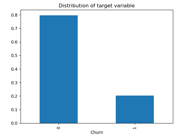
But it can happen that the positive class has a very low proportion of data points (0.2) compared to the negative class (0.8). The machine learning may not perform well with the class with less observations, leading to failing on solving the task.
To overcome this issue, there are two possibilities: undersampling the majority class and oversampling the minority class. Undersampling consists in reducing the number of samples by randomly removing some data points from the majority class, while Oversampling increases the number of observations in the minority class by adding randomly data points from the less frequent class. There is the imblearn that allows to balance the dataset with few lines of code:
# undersampling
from imblearn.over_sampling import RandomUnderSampler,RandomOverSampler
undersample = RandomUnderSampler(sampling_strategy='majority')
X_train, y_train = undersample.fit_resample(df_train.drop(['y'],axis=1),df_train['y'])
# oversampling
oversample = RandomOverSampler(sampling_strategy='minority')
X_train, y_train = oversample.fit_resample(df_train.drop(['y'],axis=1),df_train['y'])
However, removing or duplicating some of the observations can be ineffective sometimes in improving the performance of the model. It would be better to create new artificial data points in the minority class. A technique proposed to solve this issue is SMOTE, which is known for generating synthetic records in the class less represented. Like KNN, the idea is to identify k nearest neighbors of observations belonging to the minority class, based on a particular distance, like t. After a new point is generated at a random location between these k nearest neighbors. This process will keep creating new points until the dataset is completely balanced.
from imblearn.over_sampling import SMOTE
resampler = SMOTE(random_state=123)
X_train, y_train = resampler.fit_resample(df_train.drop(['y'],axis=1),df_train['y'])
I should highlight that these approaches should be applied only to resample the training set. We want that our machine model learns in a robust way and, then, we can apply it to make predictions on new data.
Final Thoughts
I hope you have found this comprehensive tutorial useful. It can be hard to start our first data science project without being aware of all these techniques. You can find all my code here.
There are surely other methods I didn’t cover in the article, but I preferred to focus on the most popular and known ones. Do you have other suggestions? Drop them in the comments if you have insightful suggestions.
Useful resources:
- A Practical Guide for Exploratory Data Analysis
- Which models require normalized data?
- Random Oversampling and Undersampling for Imbalanced Classification
Eugenia Anello is currently a research fellow at the Department of Information Engineering of the University of Padova, Italy. Her research project is focused on Continual Learning combined with Anomaly Detection.