R squared Does Not Measure Predictive Capacity or Statistical Adequacy
The fact that R-squared shouldn't be used for deciding if you have an adequate model is counter-intuitive and is rarely explained clearly. This demonstration overviews how R-squared goodness-of-fit works in regression analysis and correlations, while showing why it is not a measure of statistical adequacy, so should not suggest anything about future predictive performance.
By Georgi Georgiev, Webfocus.
The R-squared Goodness-of-Fit measure is one of the most widely available statistics accompanying the output of regression analysis in statistical software. Perhaps partially due to its widespread availability, it is also one of the most often misunderstood ones.
First, a brief refresher on R-squared (R2). In a regression with a single independent variable R2 is calculated as the ratio between the variation explained by the model and the total observed variation. It is often called the coefficient of determination and can be interpreted as the proportion of variation explained by the posed predictor. In such a case, it is equivalent to the square of the correlation coefficient of the observed and fitted values of the variable. In multiple regression, it is called the coefficient of multiple determination and is often calculated using an adjustment that penalizes its value depending on the number of predictors used.
In neither of these cases, however, does R2 measure whether the right model was chosen, and consequently, it does not measure the predictive capacity of the obtained fit. This is correctly noted in multiple sources, but few make it clear that statistical adequacy is a prerequisite of correctly interpreting a coefficient of determination. Exceptions include Spanos 2019 [1] wherein one can read “It is important to emphasize that the above statistics [R-squared and others] are meaningful only in the case where the estimated linear regression model […] is statistically adequate,” and Hagquist & Stenbeck (1998).[2] It is even rarer to see examples of why that is the case with an exception being Ford 2015.[3]
The present article includes a broader set of examples that elucidate the role and limitations of the coefficient of determination. To keep it manageable, only single variable regression is examined.
The Appeal of R-squared
First, let us examine the utility of R2 and to see why it is so easy to incorrectly interpret it as a measure of statistical adequacy and predictive accuracy when it is neither. Using a comparison with the simple linear correlation coefficient will help us understand why it behaves the way it does.
Figure 1 below is based on extracted data from 32 price offers for second-hand cars of one high-end model. The idea is to examine the relationship between car age (x-axis) and price (y-axis, in my local currency unit).

Figure 1.
Entering the data into a correlation coefficient calculator, we obtain a Pearson’s r of -0.8978 (p-value 0 to the 8th decimal place, 95%CI: -0.9493, -0.7992). This results in a comfortable R2 of 0.8059, which would, in fact, be considered high by many standards. The correlation calculation is equivalent to running a linear regression.
Eyeballing the fit makes it obvious that it can likely be improved by choosing a non-linear relationship from the exponential family as such:
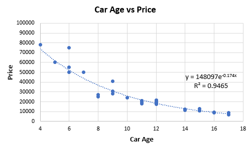
Figure 2.
The fit obtained with the regression equation shown in Figure 2 above has an R2 value of 0.9465, and so one is compelled to replace the linear with the exponential model. As the exponential model explains more of the variance, one might think it is a better representation of the underlying data generating mechanism, and perhaps this also means it will have better predictive accuracy. That is the intuitive appeal of using R-squared to choose between one model and another. However, this is not necessarily so as the next parts will demonstrate.
Different Underlying Model, Same R-squared?
What if told you that you can get the same R2 statistic for a linear regression of two distinct datasets while knowing that the underlying model is quite different in each set? This can be demonstrated by a simple simulation. The following R code produces predictor and response values based on two separate true models – one is linear, and the other is exponential:
set.seed(1);                           # set seed for replicability
x <- seq(1,10,length.out = 1000)       # predictor values
y <- 1 + 1.5*x + rnorm(1000, 0, 0.80)  # response values produced as a linear function of x and random noise with sd of 0.649
summary(lm(y ~ x))$r.squared           # print R-squared for the linear model
y <- x^2 + rnorm(1000, 0, 0.80)        # response values produced as an exponential function of x and random noise with sd of 1.377
summary(lm(y ~ x))$r.squared           # print R-squared for the exponential model
The result of the linear model fit is R2 = 0.957 for both. However, we know that one set of data comes from a linear dependence and another from an exponential one. This can be further explored using the plots of the response variable y, as shown in Figure 3.
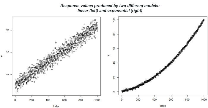
Figure 3.
If one uses an R-squared threshold to accept a model, they would be equally likely to accept a linear model for both dependencies.
Despite the same R-squared statistic produced, the predictive validity would be rather different depending on what the true dependency is. If it is truly linear, then the predictive accuracy would be quite good. Otherwise, it will be much poorer. In this sense, R-Squared is not a good measure of predictive error. The standard error would have been a much better guide being roughly seven times smaller in the first case.
Low R-squared Doesn’t Necessarily Mean an Inadequate Statistical Model
In the first example, the standard deviation of the random noise was kept the same, and we changed only the type of dependency. However, the coefficient of determination is significantly influenced by the dispersion of the random error term, and this is what we will examine next.
The code below produces simulated R2 values for different levels of the standard deviation of the error term for y while keeping the type of dependency the same. The data is generated with an adequate model for the error term, and the relationship is linear. It satisfies the simple regression model on all accounts: normality, zero mean, homoskedasticity, no autocorrelation, and no collinearity as just a single variable is involved.
r2 <- function(sd){
  x <- seq(1,10,length.out = 1000)       # predictor values
  y <- 2 + 1.2*x + rnorm(1000,0,sd = sd) # response values produced as a linear function of x and random noise with sd of sd
  summary(lm(y ~ x))$r.squared           # print R-squared
}

sds <- seq(0.5,40,length.out = 40)       # generate sd values with a step of 0.5
res <- sapply(sds, r2)                   # calculate the function with each sd value
plot(res ~ sds, type="b", main="R-squared for different values of Sigma", xlab="Sigma (Standard Deviation)", ylab="Average R-squared")
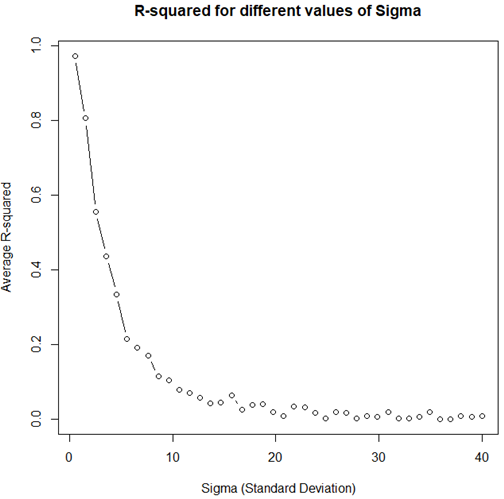
Figure 4.
Even though the statistical model satisfies all requirements and is therefore well specified, with increasing variance in the error term, the R2 value tends to zero. The above is a demonstration of why it cannot be used as a measure of statistical inadequacy.
High R-squared Doesn’t Necessarily Mean an Adequate Statistical Model
The opposite to the above scenario can happen if the model is miss-specified yet the standard deviation is sufficiently small. This will tend to produce high R2 values as demonstrated by running the code below.
r2 <- function(sd){
  x <- seq(1,10,length.out = 1000)       # predictor values
  y <- x^2 + rnorm(1000,0,sd = sd)       # response values produced as a linear function of x and random noise with sd of sd
  summary(lm(y ~ x))$r.squared           # print R-squared
}

sds <- seq(0.5,40,length.out = 40)       # genearte sd values with a step of 0.5
res <- sapply(sds, r2)                   # calculate the function with each sd value
plot(res ~ sds, type="b", main="R-squared for different values of Sigma", xlab="Sigma (Standard Deviation)", ylab="Average R-squared")
It should produce a plot like the one shown on Figure 5.
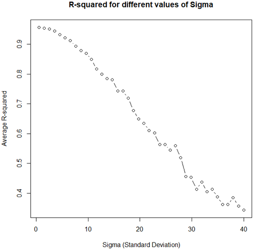
Figure 5.
As evident, even with a decidedly non-linear underlying model, very high R-squared values can be observed for a wide range of sigma values. This means that even arbitrarily high values of the statistic cannot necessarily be taken as evidence for model adequacy.
In conclusion
Hopefully, the above examples serve as a sufficient illustration of the dangers of over-interpreting the coefficient of determination. While it is a measure of goodness-of-fit, it only gains meaning if the model is adequate with respect to the underlying mechanism generating the data. Using it as a measure of model adequacy is not warranted, and to the extent to which homing in on the correct model affects or predictive error, it is not a measure of it either. Whether that leaves any useful place for it whatsoever is still a matter of debate.
References:
[1] Spanos A. (2019). “Probability Theory and Statistical Inference: Empirical Modeling with Observational Data.” Cambridge University Press. p.635
[2] Hagquist, C., Stenbeck, M. (1998) “Goodness of Fit in Regression Analysis – R 2 and G 2 Reconsidered.” Quality and Quantity. 32, pp.229–245
[3] Ford C. (2015). “Is R-squared Useless?” https://data.library.virginia.edu/is-r-squared-useless/
Bio: Georgi Georgiev is the author of Statistical Methods in Online A/B Testing, Founder of Analytics-Toolkit.com, and Owner & Manager of Web Focus LLC.
Related: