Spam Filter in Python: Naive Bayes from Scratch
In this blog post, learn how to build a spam filter using Python and the multinomial Naive Bayes algorithm, with a goal of classifying messages with a greater than 80% accuracy.
By Alex Olteanu, Data Scientist at Dataquest
In this blog post, we're going to build a spam filter using Python and the multinomial Naive Bayes algorithm. Our goal is to code a spam filter from scratch that classifies messages with an accuracy greater than 80%.
To build our spam filter, we'll use a dataset of 5,572 SMS messages. Tiago A. Almeida and José María Gómez Hidalgo put together the dataset, you can download it from the UCI Machine Learning Repository.
We're going to focus on the Python implementation throughout the post, so we'll assume that you are already familiar with multinomial Naive Bayes and conditional proability.
If you need to fill in any gaps before moving forward, Dataquest has a course that covers both conditional probability and multinomial Naive Bayes, as well as a broad variety of other course you could use to fill in gaps in your knowledge and earn a data science certificate.
Exploring the Dataset
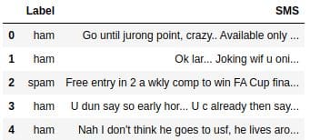
Let's start by opening the SMSSpamCollection file with the read_csv() function from the pandas package. We're going to use:
sep='\t'because the data points are tab separatedheader=Nonebecause the dataset doesn't have a header rownames=['Label', 'SMS']to name the columns
import pandas as pd

sms_spam = pd.read_csv('SMSSpamCollection', sep='\t',
header=None, names=['Label', 'SMS'])

print(sms_spam.shape)
sms_spam.head()
(5572, 2)
Below, we see that about 87% of the messages are ham (non-spam), and the remaining 13% are spam. This sample looks representative, since in practice most messages that people receive are ham.
sms_spam['Label'].value_counts(normalize=True)
ham     0.865937

spam    0.134063

Name: Label, dtype: float64
Training and Test Set
We're now going to split our dataset into a training set and a test set. We'll use 80% of the data for training and the remaining 20% for testing.
We'll randomize the entire dataset before splitting to ensure that spam and ham messages are spread properly throughout the dataset.
# Randomize the dataset
data_randomized = sms_spam.sample(frac=1, random_state=1)

# Calculate index for split
training_test_index = round(len(data_randomized) * 0.8)

# Split into training and test sets
training_set = data_randomized[:training_test_index].reset_index(drop=True)
test_set = data_randomized[training_test_index:].reset_index(drop=True)

print(training_set.shape)
print(test_set.shape)
(4458, 2)

(1114, 2)
We'll now analyze the percentage of spam and ham messages in the training and test sets. We expect the percentages to be close to what we have in the full dataset, where about 87% of the messages are ham, and the remaining 13% are spam.
training_set['Label'].value_counts(normalize=True)
ham     0.86541

spam    0.13459

Name: Label, dtype: float64
test_set['Label'].value_counts(normalize=True)
ham     0.868043

spam    0.131957

Name: Label, dtype: float64
The results look great! We'll now move on to cleaning the dataset.
Data Cleaning
When a new message comes in, our multinomial Naive Bayes algorithm will make the classification based on the results it gets to these two equations below, where "w1" is the first word, and w1,w2, ..., wn is the entire message:

If P(Spam | w1,w2, ..., wn) is greater than P(Ham | w1,w2, ..., wn), then the message is spam.
To calculate P(wi|Spam) and P(wi|Ham), we need to use separate equations:
Let's clarify some of the terms in these equations:
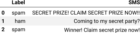
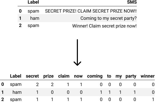
To calculate all these probabilities, we'll first need to perform a bit of data cleaning to bring the data into a format that allows us to easily extract all the information we need. Right now, our training and test sets have this format (the messages below are fictitious to make the example easier to understand):
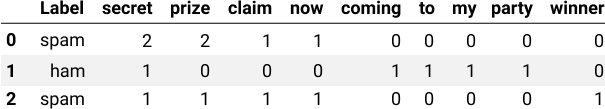
- The
SMScolumn is replaced by a series of new columns that represent unique words from the vocabulary — the vocabulary is the set of unique words from all of our sentences. - Each row describes a single message. The first row has the values
spam, 2, 2, 1, 1, 0, 0, 0, 0, 0, which tell us that:- The message is spam.
- The word "secret" occurs two times inside the message.
- The word "prize" occurs two times inside the message.
- The word "claim" occurs one time inside the message.
- The word "now" occurs one time inside the message.
- The words "coming," "to," "my," "party," and "winner" occur zero times inside the message.
- All words in the vocabulary are in lowercase, so "SECRET" and "secret" are considered the same word.
- The order of words in the original sentences is lost.
- Punctuation is no longer taken into account (for instance, we can't look at the table and conclude that the first message initially had two exclamation marks).
Letter Case and Punctuation
Let's begin the data cleaning process by removing the punctuation and making all the words lowercase.
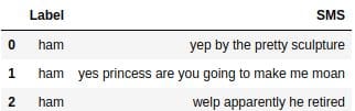
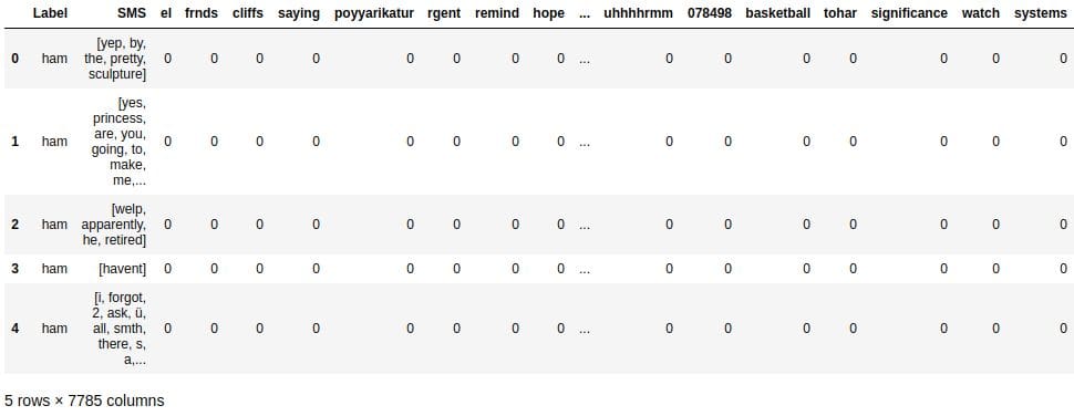
# Before cleaning
training_set.head(3)
# After cleaning
training_set['SMS'] = training_set['SMS'].str.replace(
   '\W', ' ') # Removes punctuation
training_set['SMS'] = training_set['SMS'].str.lower()
training_set.head(3)
Creating the Vocabulary
Let's now create the vocabulary, which in this context means a list with all the unique words in our training set. In the code below:
- We transform each message in the
SMScolumn into a list by splitting the string at the space character — we're using theSeries.str.split()method. - We initiate an empty list named
vocabulary. - We iterate over the transformed
SMScolumn.- Using a nested loop, we iterate over each message in the
SMScolumn and append each string (word) to thevocabularylist.
- Using a nested loop, we iterate over each message in the
- We transform the
vocabularylist into a set using theset()function. This will remove the duplicates from thevocabularylist. - We transform the
vocabularyset back into a list using thelist()function.
training_set['SMS'] = training_set['SMS'].str.split()

vocabulary = []
for sms in training_set['SMS']:
   for word in sms:
      vocabulary.append(word)

vocabulary = list(set(vocabulary))
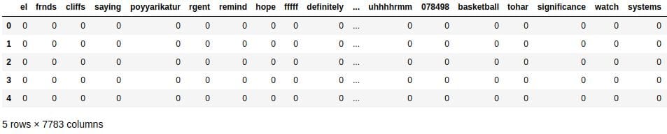
It looks like there are 7,783 unique words in all the messages of our training set.
len(vocabulary)
7783
The Final Training Set
We're now going to use the vocabulary we just created to make the data transformation we want.
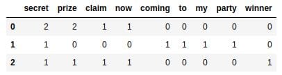
For instance, to create the table we see above, we can use this dictionary:
word_counts_per_sms = {'secret': [2,1,1],
                       'prize': [2,0,1],
                       'claim': [1,0,1],
                       'now': [1,0,1],
                       'coming': [0,1,0],
                       'to': [0,1,0],
                       'my': [0,1,0],
                       'party': [0,1,0],
                       'winner': [0,0,1]
                      }

word_counts = pd.DataFrame(word_counts_per_sms)
word_counts.head()
To create the dictionary we need for our training set, we can use the code below:
- We start by initializing a dictionary named
word_counts_per_sms, where each key is a unique word (a string) from the vocabulary, and each value is a list of the length of the training set, where each element in that list is a0.- The code
[0] * 5outputs[0, 0, 0, 0, 0]. So the code[0] * len(training_set['SMS'])outputs a list of the length oftraining_set['SMS'].
- The code
- We loop over
training_set['SMS']using theenumerate()function to get both the index and the SMS message (indexandsms).- Using a nested loop, we loop over
sms(wheresmsis a list of strings, where each string represents a word in a message).- We increment
word_counts_per_sms[word][index]by1.
- We increment
- Using a nested loop, we loop over
word_counts_per_sms = {unique_word: [0] * len(training_set['SMS']) for unique_word in vocabulary}

for index, sms in enumerate(training_set['SMS']):
   for word in sms:
      word_counts_per_sms[word][index] += 1
Now that we have the dictionary we need, let's do the final transformations to our training set.
word_counts = pd.DataFrame(word_counts_per_sms)
word_counts.head()
The Label column is missing, so we'll use the pd.concat() function to concatenate the DataFrame we just built with the DataFrame containing the training set. This way, we'll also have the Label and the SMS columns.
training_set_clean = pd.concat([training_set, word_counts], axis=1)
training_set_clean.head()
Calculating Constants First
Now that we're done with cleaning the training set, we can begin coding the spam filter. The multinomial Naive Bayes algorithm will need to answer these two probability questions to be able to classify new messages:
Also, to calculate P(wi|Spam) and P(wi|Ham) inside the formulas above, we'll need to use these equations:
Some of the terms in the four equations above will have the same value for every new message. We can calculate the value of these terms once and avoid doing the computations again when a new messages comes in. As a start, let's first calculate:
- P(Spam) and P(Ham)
- NSpam, NHam, NVocabulary
It's important to note that:
- NSpam is equal to the number of words in all the spam messages — it's not equal to the number of spam messages, and it's not equal to the total number of unique words in spam messages.
- NHam is equal to the number of words in all the non-spam messages — it's not equal to the number of non-spam messages, and it's not equal to the total number of unique words in non-spam messages.
We'll also use Laplace smoothing and set .
# Isolating spam and ham messages first
spam_messages = training_set_clean[training_set_clean['Label'] == 'spam']
ham_messages = training_set_clean[training_set_clean['Label'] == 'ham']

# P(Spam) and P(Ham)
p_spam = len(spam_messages) / len(training_set_clean)
p_ham = len(ham_messages) / len(training_set_clean)

# N_Spam
n_words_per_spam_message = spam_messages['SMS'].apply(len)
n_spam = n_words_per_spam_message.sum()

# N_Ham
n_words_per_ham_message = ham_messages['SMS'].apply(len)
n_ham = n_words_per_ham_message.sum()

# N_Vocabulary
n_vocabulary = len(vocabulary)

# Laplace smoothing
alpha = 1
Calculating Parameters
Now that we have the constant terms calculated above, we can move on with calculating the parameters P(wi|Spam) and P(wi|Ham).
P(wi|Spam) and P(wi|Ham) will vary depending on the individual words. For instance, P("secret"|Spam) will have a certain probability value, while P("cousin"|Spam) or P("lovely"|Spam) will most likely have other values.
Therefore, each parameter will be a conditional probability value associated with each word in the vocabulary.
The parameters are calculated using these two equations:
# Initiate parameters
parameters_spam = {unique_word:0 for unique_word in vocabulary}
parameters_ham = {unique_word:0 for unique_word in vocabulary}

# Calculate parameters
for word in vocabulary:
   n_word_given_spam = spam_messages[word].sum() # spam_messages already defined
   p_word_given_spam = (n_word_given_spam + alpha) / (n_spam + alpha*n_vocabulary)
   parameters_spam[word] = p_word_given_spam

   n_word_given_ham = ham_messages[word].sum() # ham_messages already defined
   p_word_given_ham = (n_word_given_ham + alpha) / (n_ham + alpha*n_vocabulary)
   parameters_ham[word] = p_word_given_ham
Classifying A New Message
Now that we have all our parameters calculated, we can start creating the spam filter. The spam filter is understood as a function that:
- Takes in as input a new message (w1, w2, ..., wn).
- Calculates P(Spam|w1, w2, ..., wn) and P(Ham|w1, w2, ..., wn).
- Compares the values of P(Spam|w1, w2, ..., wn) and P(Ham|w1, w2, ..., wn), and:
- If P(Ham|w1, w2, ..., wn) > P(Spam|w1, w2, ..., wn), then the message is classified as ham.
- If P(Ham|w1, w2, ..., wn) < P(Spam|w1, w2, ..., wn), then the message is classified as spam.
- If P(Ham|w1, w2, ..., wn) = P(Spam|w1, w2, ..., wn), then the algorithm may request human help.
Note that some new messages will contain words that are not part of the vocabulary. We will simply ignore these words when we're calculating the probabilities.
Let's start by writing a first version of this function. For the classify() function below, notice that:
- The input variable
messageneeds to be a string. - We perform a bit of data cleaning on the string
message:- We remove the punctuation using the
re.sub()function. - We bring all letters to lower case using the
str.lower()method. - We split the string at the space character and transform it into a Python list using the
str.split()method.
- We remove the punctuation using the
- We calculate
p_spam_given_messageandp_ham_given_message. - We compare
p_spam_given_messagewithp_ham_given_messageand then print a classification label.
import re

def classify(message):
   '''
   message: a string
   '''

   message = re.sub('\W', ' ', message)
   message = message.lower().split()

   p_spam_given_message = p_spam
   p_ham_given_message = p_ham

   for word in message:
      if word in parameters_spam:
         p_spam_given_message *= parameters_spam[word]

      if word in parameters_ham:
         p_ham_given_message *= parameters_ham[word]

   print('P(Spam|message):', p_spam_given_message)
   print('P(Ham|message):', p_ham_given_message)

   if p_ham_given_message > p_spam_given_message:
      print('Label: Ham')
   elif p_ham_given_message < p_spam_given_message:
      print('Label: Spam')
   else:
      print('Equal proabilities, have a human classify this!')
We'll now test the spam filter on two new messages. One message is obviously spam, and the other is obviously ham.
classify('WINNER!! This is the secret code to unlock the money: C3421.')
P(Spam|message): 1.3481290211300841e-25

P(Ham|message): 1.9368049028589875e-27

Label: Spam
classify("Sounds good, Tom, then see u there")
P(Spam|message): 2.4372375665888117e-25

P(Ham|message): 3.687530435009238e-21

Label: Ham
Measuring the Spam Filter's Accuracy
The two results look promising, but let's see how well the filter does on our test set, which has 1,114 messages.
We'll start by writing a function that returns classification labels instead of printing them.
def classify_test_set(message):
   '''
   message: a string
   '''

   message = re.sub('\W', ' ', message)
   message = message.lower().split()

   p_spam_given_message = p_spam
   p_ham_given_message = p_ham

   for word in message:
      if word in parameters_spam:
         p_spam_given_message *= parameters_spam[word]

      if word in parameters_ham:
         p_ham_given_message *= parameters_ham[word]

   if p_ham_given_message > p_spam_given_message:
      return 'ham'
   elif p_spam_given_message > p_ham_given_message:
      return 'spam'
   else:
      return 'needs human classification'
Now that we have a function that returns labels instead of printing them, we can use it to create a new column in our test set.
test_set['predicted'] = test_set['SMS'].apply(classify_test_set)
test_set.head()
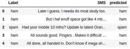
We can compare the predicted values with the actual values to measure how good our spam filter is with classifying new messages. To make the measurement, we'll use accuracy as a metric:
correct = 0
total = test_set.shape[0]

for row in test_set.iterrows():
   row = row[1]
   if row['Label'] == row['predicted']:
      correct += 1

print('Correct:', correct)
print('Incorrect:', total - correct)
print('Accuracy:', correct/total)
Correct: 1100

Incorrect: 14

Accuracy: 0.9874326750448833
The accuracy is close to 98.74%, which is really good. Our spam filter looked at 1,114 messages that it hasn't seen in training, and classified 1,100 correctly.
Next Steps
In this blog post, we managed to code a spam filter for SMS messages using the multinomial Naive Bayes algorithm. The filter had an accuracy of 98.74% on the test set we used, which is a promising result. Our initial goal was an accuracy of over 80%, and we managed to accomplish that.
Some of the next steps you can take include:
- Analyzing the 14 messages that were classified incorrectly and trying to figure out why the algorithm classified them incorrectly
- Making the filtering process more complex by making the algorithm sensitive to letter case
Bio: Alex Olteanu is a Data Scientist at Dataquest.
Related: