Linear Regression from Scratch with NumPy
Mastering the Basics of Linear Regression and Fundamentals of Gradient Descent and Loss Minimization.
Image by Author
Motivation
Linear Regression is one of the most fundamental tools in machine learning. It is used to find a straight line that fits our data well. Even though it only works with simple straight-line patterns, understanding the math behind it helps us understand Gradient Descent and Loss Minimization methods. These are important for more complicated models used in all machine learning and deep learning tasks.
In this article, we'll roll up our sleeves and build Linear Regression from scratch using NumPy. Instead of using abstract implementations such as those provided by Scikit-Learn, we will start from the basics.
Dataset
We generate a dummy dataset using Scikit-Learn methods. We only use a single variable for now, but the implementation will be general that can train on any number of features.
The make_regression method provided by Scikit-Learn generates random linear regression datasets, with added Gaussian noise to add some randomness.
X, y = datasets.make_regression(
        n_samples=500, n_features=1, noise=15, random_state=4)
We generate 500 random values, each with 1 single feature. Therefore, X has shape (500, 1) and each of the 500 independent X values, has a corresponding y value. So, y also has shape (500, ).
Visualized, the dataset looks as follows:
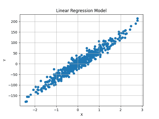
Image by Author
We aim to find a best-fit line that passes through the center of this data, minimizing the average difference between the predicted and original y values.
Intuition
The general equation for a linear line is:
y = m*X + b
X is numeric, single-valued. Here m and b represent the gradient and y-intercept (or bias). These are unknowns, and varying values of these can generate different lines. In machine learning, X is dependent on the data, and so are the y values. We only have control over m and b, that act as our model parameters. We aim to find optimal values of these two parameters, that generate a line that minimizes the difference between predicted and actual y values.
This extends to the scenario where X is multi-dimensional. In that case, the number of m values will equal the number of dimensions in our data. For example, if our data has three different features, we will have three different m values, called weights.
The equation will now become:
y = w1*X1 + w2*X2 + w3*X3 + b
This can then extend to any number of features.
But how do we know the optimal values of our bias and weight values? Well, we don’t. But we can iteratively find it out using Gradient Descent. We start with random values and change them slightly for multiple steps until we get close to the optimal values.
First, let us initialize Linear Regression, and we will go over the optimization process in greater detail later.
Initialize Linear Regression Class
import numpy as np


class LinearRegression:
    def __init__(self, lr: int = 0.01, n_iters: int = 1000) -> None:
        self.lr = lr
        self.n_iters = n_iters
        self.weights = None
        self.bias = None
We use a learning rate and number of iterations hyperparameters, that will be explained later. The weights and biases are set to None because the number of weight parameters depends on the input features within the data. We do not have access to the data yet, so we initialize them to None for now.
The Fit Method
In the fit method, we are provided with data and their associated values. We can now use these, to initialize our weights, and then train the model to find optimal weights.
def fit(self, X, y):
        num_samples, num_features = X.shape     # X shape [N, f]
        self.weights = np.random.rand(num_features)  # W shape [f, 1]
        self.bias = 0
The independent feature X will be a NumPy array of shape (num_samples, num_features). In our case, the shape of X is (500, 1). Each row in our data will have an associated target value, so y is also of shape (500,) or (num_samples).
We extract this and randomly initialize the weights given the number of input features. So now our weights are also a NumPy array of size (num_features, ). Bias is a single value initialized to zero.
Predicting Y Values
We use the line equation discussed above to calculate predicted y values. However, instead of an iterative approach to sum all values, we can follow a vectorized approach for faster computation. Given that the weights and X values are NumPy arrays, we can use matrix multiplication to get predictions.
X has shape (num_samples, num_features) and weights have shape (num_features, ). We want the predictions to be of shape (num_samples, ) matching the original y values. Therefore we can multiply X with weights, or (num_samples, num_features) x (num_features, ) to obtain predictions of shape (num_samples, ).
The bias value is added at the end of each prediction. This can simply be implemented in a single line.
# y_pred shape should be N, 1
y_pred = np.dot(X, self.weights) + self.bias
However, are these predictions correct? Obviously not. We are using randomly initialized values for the weights and bias, so the predictions will also be random.
How do we get the optimal values? Gradient Descent.
Loss Function and Gradient Descent
Now that we have both predicted and target y values, we can find the difference between both values. Mean Square Error (MSE) is used to compare real-valued numbers. The equation is as follows:
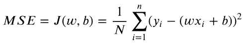
We only care about the absolute difference between our values. A prediction higher than the original value is as bad as a lower prediction. So we square the difference between our target value and predictions, to convert negative differences to positive. Moreover, this penalizes a larger difference between targets and predictions, as higher differences squared will contribute more to the final loss.
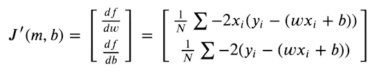
For our predictions to be as close to original targets as possible, we now try to minimize this function. The loss function will be minimum, where the gradient is zero. As we can only optimize our weights and bias values, we take the partial derivates of the MSE function with respect to weights and bias values.
We then optimize our weights given the gradient values, using Gradient Descent.
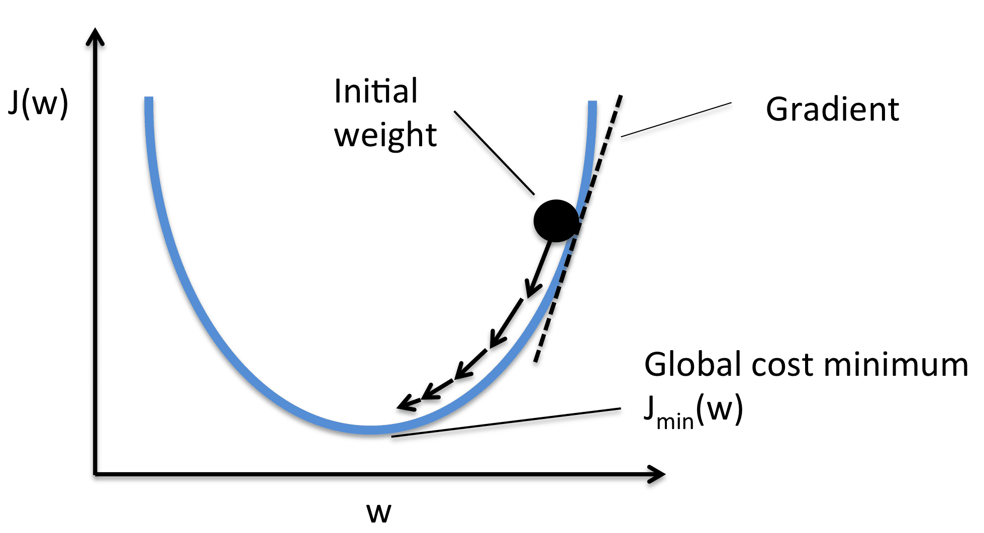
Image from Sebasitan Raschka
We take the gradient with respect to each weight value and then move them to the opposite of the gradient. This pushes the the loss towards minimum. As per the image, the gradient is positive, so we decrease the weight. This pushes the J(W) or loss towards the minimum value. Therefore, the optimization equations look as follows:
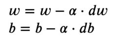
The learning rate (or alpha) controls the incremental steps shown in the image. We only make a small change in the value, for stable movement towards the minimum.
Implementation
If we simplify the derivate equation using basic algebraic manipulation, this becomes very simple to implement.
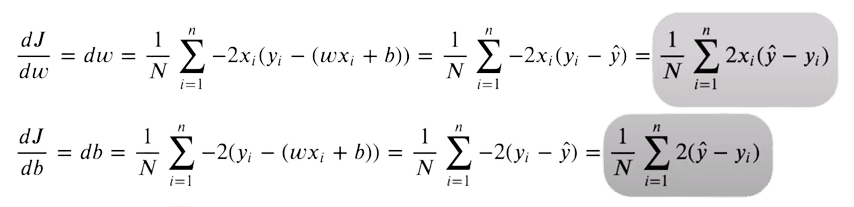
For the derivate, we implement this using two lines of code:
# X -> [ N, f ]
# y_pred -> [ N ]
# dw -> [ f ]
dw = (1 / num_samples) * np.dot(X.T, y_pred - y)
db = (1 / num_samples) * np.sum(y_pred - y)
dw is again of shape (num_features, ) So we have a separate derivate value for each weight. We optimize them separately. db has a single value.
To optimize the values now, we move the values in the opposite direction of the gradient using basic subtraction.
self.weights = self.weights - self.lr * dw
self.bias = self.bias - self.lr * db
Again, this is only a single step. We only make a small change to the randomly initialized values. We now repeatedly perform the same steps, to converge towards a minimum.
The complete loop is as follows:
for i in range(self.n_iters):

            # y_pred shape should be N, 1
            y_pred = np.dot(X, self.weights) + self.bias

            # X -> [N,f]
            # y_pred -> [N]
            # dw -> [f]
            dw = (1 / num_samples) * np.dot(X.T, y_pred - y)
            db = (1 / num_samples) * np.sum(y_pred - y)

            self.weights = self.weights - self.lr * dw
            self.bias = self.bias - self.lr * db
Prediction
We predict the same way as we did during training. However, now we have the optimal set of weights and biases. The predicted values should now be close to the original values.
def predict(self, X):
        return np.dot(X, self.weights) + self.bias
Results
With randomly initialized weights and bias, our predictions were as follows:
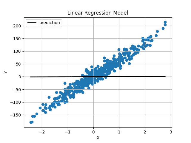
Image by Author
Weight and bias were initialized very close to 0, so we obtain a horizontal line. After training the model for 1000 iterations, we get this:
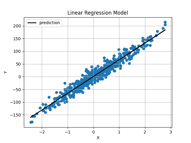
Image by Author
The predicted line passes right through the center of our data and seems to be the best-fit line possible.
Conclusion
You have now implemented Linear Regression from scratch. The complete code is also available on GitHub.
import numpy as np


class LinearRegression:
    def __init__(self, lr: int = 0.01, n_iters: int = 1000) -> None:
        self.lr = lr
        self.n_iters = n_iters
        self.weights = None
        self.bias = None

    def fit(self, X, y):
        num_samples, num_features = X.shape     # X shape [N, f]
        self.weights = np.random.rand(num_features)  # W shape [f, 1]
        self.bias = 0

        for i in range(self.n_iters):

            # y_pred shape should be N, 1
            y_pred = np.dot(X, self.weights) + self.bias

            # X -> [N,f]
            # y_pred -> [N]
            # dw -> [f]
            dw = (1 / num_samples) * np.dot(X.T, y_pred - y)
            db = (1 / num_samples) * np.sum(y_pred - y)

            self.weights = self.weights - self.lr * dw
            self.bias = self.bias - self.lr * db

        return self

    def predict(self, X):
        return np.dot(X, self.weights) + self.bias
Muhammad Arham is a Deep Learning Engineer working in Computer Vision and Natural Language Processing. He has worked on the deployment and optimizations of several generative AI applications that reached the global top charts at Vyro.AI. He is interested in building and optimizing machine learning models for intelligent systems and believes in continual improvement.